

2.5 Particle Velocimetry Measurements
79
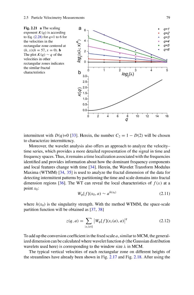
Fig. 2.21 a The scaling
exponent K (q) is according
to Eq. (2.28) for q=1 to 6 for
the velocities in the
rectangular zone centered at
(h, x)(h = 57, x = 0). b
The plot K (q) ∼ q of the
velocities in other
rectangular zones indicates
the similar fractal
characteristics
intermittent with D(q)=0 [33]. Herein, the number C 2 = 1 − D(2) will be chosen
to characterize intermittency.
Moreover, the wavelet analysis also offers an approach to analyze the velocity–
time series, which provides a more detailed representation of the signal in time and
frequency spaces. Thus, it remains a time localization associated with the frequencies
identified and provides information about how the dominant frequency components
and local features change with time [34]. Herein, the Wavelet Transform Modulus
Maxima (WTMM) [34, 35] is used to analyze the fractal dimension of the data for
detecting intermittent patterns by partitioning the time and scale domains into fractal
dimension regions [36]. The WT can reveal the local characteristics of f (x) at a
point x 0 :
W φ [ f ](x 0 , a) ∼ a
h(x 0 )
(2.11)
where h(x 0 ) is the singularity strength. With the method WTMM, the space-scale
partition function will be obtained as [37, 38]
z(q, a) =
|x i (a)|
W φ [ f ](x i (a), a)
q
(2.12)
To add up the conversion coefficient in the fixed scale a, similar to MCM, the generalized dimension can be calculated where wavelet function φ (the Gaussian distribution
wavelets used here) is corresponding to the window size λ in MCM.
The typical vertical velocities of each rectangular zone on different heights of
the streamlines have already been shown in Fig. 2.17 and Fig. 2.18. After using the
79
Fig. 2.21 a The scaling
exponent K (q) is according
to Eq. (2.28) for q=1 to 6 for
the velocities in the
rectangular zone centered at
(h, x)(h = 57, x = 0). b
The plot K (q) ∼ q of the
velocities in other
rectangular zones indicates
the similar fractal
characteristics
intermittent with D(q)=0 [33]. Herein, the number C 2 = 1 − D(2) will be chosen
to characterize intermittency.
Moreover, the wavelet analysis also offers an approach to analyze the velocity–
time series, which provides a more detailed representation of the signal in time and
frequency spaces. Thus, it remains a time localization associated with the frequencies
identified and provides information about how the dominant frequency components
and local features change with time [34]. Herein, the Wavelet Transform Modulus
Maxima (WTMM) [34, 35] is used to analyze the fractal dimension of the data for
detecting intermittent patterns by partitioning the time and scale domains into fractal
dimension regions [36]. The WT can reveal the local characteristics of f (x) at a
point x 0 :
W φ [ f ](x 0 , a) ∼ a
h(x 0 )
(2.11)
where h(x 0 ) is the singularity strength. With the method WTMM, the space-scale
partition function will be obtained as [37, 38]
z(q, a) =
|x i (a)|
W φ [ f ](x i (a), a)
q
(2.12)
To add up the conversion coefficient in the fixed scale a, similar to MCM, the generalized dimension can be calculated where wavelet function φ (the Gaussian distribution
wavelets used here) is corresponding to the window size λ in MCM.
The typical vertical velocities of each rectangular zone on different heights of
the streamlines have already been shown in Fig. 2.17 and Fig. 2.18. After using the