

5.3 Discrete Modeling of Pebble Radiation
301
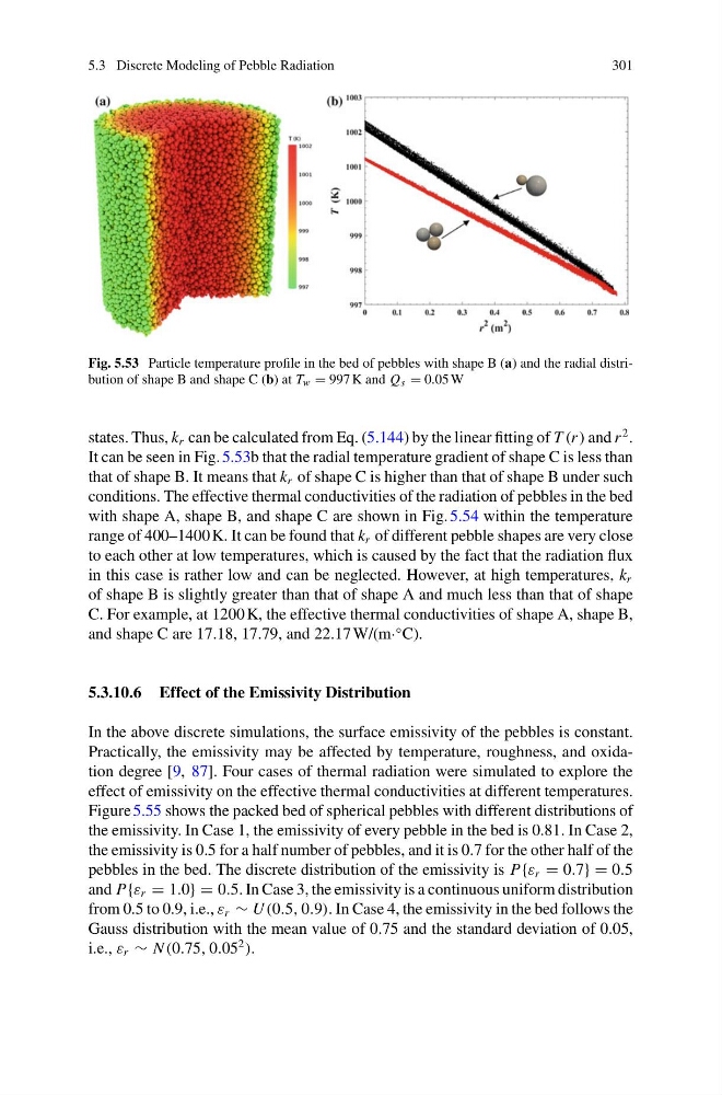
Fig. 5.53 Particle temperature profile in the bed of pebbles with shape B (a) and the radial distribution of shape B and shape C (b) at T w = 997 K and Q s = 0.05 W
states. Thus, k r can be calculated from Eq. (5.144) by the linear fitting of T (r ) and r
2 .
It can be seen in Fig. 5.53b that the radial temperature gradient of shape C is less than
that of shape B. It means that k r of shape C is higher than that of shape B under such
conditions. The effective thermal conductivities of the radiation of pebbles in the bed
with shape A, shape B, and shape C are shown in Fig. 5.54 within the temperature
range of 400–1400 K. It can be found that k r of different pebble shapes are very close
to each other at low temperatures, which is caused by the fact that the radiation flux
in this case is rather low and can be neglected. However, at high temperatures, k r
of shape B is slightly greater than that of shape A and much less than that of shape
C. For example, at 1200 K, the effective thermal conductivities of shape A, shape B,
and shape C are 17.18, 17.79, and 22.17 W/(m·
◦ C).
5.3.10.6 Effect of the Emissivity Distribution
In the above discrete simulations, the surface emissivity of the pebbles is constant.
Practically, the emissivity may be affected by temperature, roughness, and oxidation degree [9, 87]. Four cases of thermal radiation were simulated to explore the
effect of emissivity on the effective thermal conductivities at different temperatures.
Figure 5.55 shows the packed bed of spherical pebbles with different distributions of
the emissivity. In Case 1, the emissivity of every pebble in the bed is 0.81. In Case 2,
the emissivity is 0.5 for a half number of pebbles, and it is 0.7 for the other half of the
pebbles in the bed. The discrete distribution of the emissivity is P{ε r = 0.7} = 0.5
and P{ε r = 1.0} = 0.5. In Case 3, the emissivity is a continuous uniform distribution
from 0.5 to 0.9, i.e., ε r ∼ U (0.5, 0.9). In Case 4, the emissivity in the bed follows the
Gauss distribution with the mean value of 0.75 and the standard deviation of 0.05,
i.e., ε r ∼ N (0.75, 0.05
2
).
301
Fig. 5.53 Particle temperature profile in the bed of pebbles with shape B (a) and the radial distribution of shape B and shape C (b) at T w = 997 K and Q s = 0.05 W
states. Thus, k r can be calculated from Eq. (5.144) by the linear fitting of T (r ) and r
2 .
It can be seen in Fig. 5.53b that the radial temperature gradient of shape C is less than
that of shape B. It means that k r of shape C is higher than that of shape B under such
conditions. The effective thermal conductivities of the radiation of pebbles in the bed
with shape A, shape B, and shape C are shown in Fig. 5.54 within the temperature
range of 400–1400 K. It can be found that k r of different pebble shapes are very close
to each other at low temperatures, which is caused by the fact that the radiation flux
in this case is rather low and can be neglected. However, at high temperatures, k r
of shape B is slightly greater than that of shape A and much less than that of shape
C. For example, at 1200 K, the effective thermal conductivities of shape A, shape B,
and shape C are 17.18, 17.79, and 22.17 W/(m·
◦ C).
5.3.10.6 Effect of the Emissivity Distribution
In the above discrete simulations, the surface emissivity of the pebbles is constant.
Practically, the emissivity may be affected by temperature, roughness, and oxidation degree [9, 87]. Four cases of thermal radiation were simulated to explore the
effect of emissivity on the effective thermal conductivities at different temperatures.
Figure 5.55 shows the packed bed of spherical pebbles with different distributions of
the emissivity. In Case 1, the emissivity of every pebble in the bed is 0.81. In Case 2,
the emissivity is 0.5 for a half number of pebbles, and it is 0.7 for the other half of the
pebbles in the bed. The discrete distribution of the emissivity is P{ε r = 0.7} = 0.5
and P{ε r = 1.0} = 0.5. In Case 3, the emissivity is a continuous uniform distribution
from 0.5 to 0.9, i.e., ε r ∼ U (0.5, 0.9). In Case 4, the emissivity in the bed follows the
Gauss distribution with the mean value of 0.75 and the standard deviation of 0.05,
i.e., ε r ∼ N (0.75, 0.05
2
).