

256
5 Numerical Models for Pebble-Bed Heat Transfer
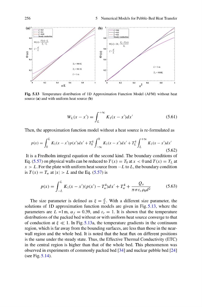
Fig. 5.13 Temperature distribution of 1D Approximation Function Model (AFM) without heat
source (a) and with uniform heat source (b)
W L (x − x
) =
+∞
L
K 1 (x − x
)dx
(5.61)
Then, the approximation function model without a heat source is re-formulated as
p(x) =
L
0
K 1 (x − x
) p(x
)dx
+ T
4
0
0
−∞
K 1 (x − x
)dx
+ T
4
L
+∞
L
K 1 (x − x
)dx
(5.62)
It is a Fredholm integral equation of the second kind. The boundary conditions of
Eq. (5.57) on physical walls can be reduced to T (x) = T 0 at x < 0 and T (x) = T L at
x > L. For the plate with uniform heat source from −L to L, the boundary condition
is T (x) = T w at |x| > L and the Eq. (5.57) is
p(x) =
L
−L
K 1 (x − x
)( p(x
) − T
4
w )dx
+ T
4
w +
Q v
πσ ε r ρ 0 d 2
(5.63)
The size parameter is defined as ξ =
d
L
. With a different size parameter, the
solutions of 1D approximation function models are given in Fig. 5.13, where the
parameters are L =1 m, α f = 0.39, and ε r = 1. It is shown that the temperature
distributions of the packed bed without or with uniform heat source converge to that
of conduction at ξ 1. In Fig. 5.13a, the temperature gradients in the continuum
region, which is far away from the bounding surfaces, are less than those in the nearwall region and the whole bed. It is noted that the heat flux on different positions
is the same under the steady state. Thus, the Effective Thermal Conductivity (ETC)
in the central region is higher than that of the whole bed. This phenomenon was
observed in experiments of commonly packed bed [34] and nuclear pebble bed [24]
(see Fig. 5.14).
5 Numerical Models for Pebble-Bed Heat Transfer
Fig. 5.13 Temperature distribution of 1D Approximation Function Model (AFM) without heat
source (a) and with uniform heat source (b)
W L (x − x
) =
+∞
L
K 1 (x − x
)dx
(5.61)
Then, the approximation function model without a heat source is re-formulated as
p(x) =
L
0
K 1 (x − x
) p(x
)dx
+ T
4
0
0
−∞
K 1 (x − x
)dx
+ T
4
L
+∞
L
K 1 (x − x
)dx
(5.62)
It is a Fredholm integral equation of the second kind. The boundary conditions of
Eq. (5.57) on physical walls can be reduced to T (x) = T 0 at x < 0 and T (x) = T L at
x > L. For the plate with uniform heat source from −L to L, the boundary condition
is T (x) = T w at |x| > L and the Eq. (5.57) is
p(x) =
L
−L
K 1 (x − x
)( p(x
) − T
4
w )dx
+ T
4
w +
Q v
πσ ε r ρ 0 d 2
(5.63)
The size parameter is defined as ξ =
d
L
. With a different size parameter, the
solutions of 1D approximation function models are given in Fig. 5.13, where the
parameters are L =1 m, α f = 0.39, and ε r = 1. It is shown that the temperature
distributions of the packed bed without or with uniform heat source converge to that
of conduction at ξ 1. In Fig. 5.13a, the temperature gradients in the continuum
region, which is far away from the bounding surfaces, are less than those in the nearwall region and the whole bed. It is noted that the heat flux on different positions
is the same under the steady state. Thus, the Effective Thermal Conductivity (ETC)
in the central region is higher than that of the whole bed. This phenomenon was
observed in experiments of commonly packed bed [34] and nuclear pebble bed [24]
(see Fig. 5.14).