

5.2 Continuum Modeling of Pebble Radiation
255
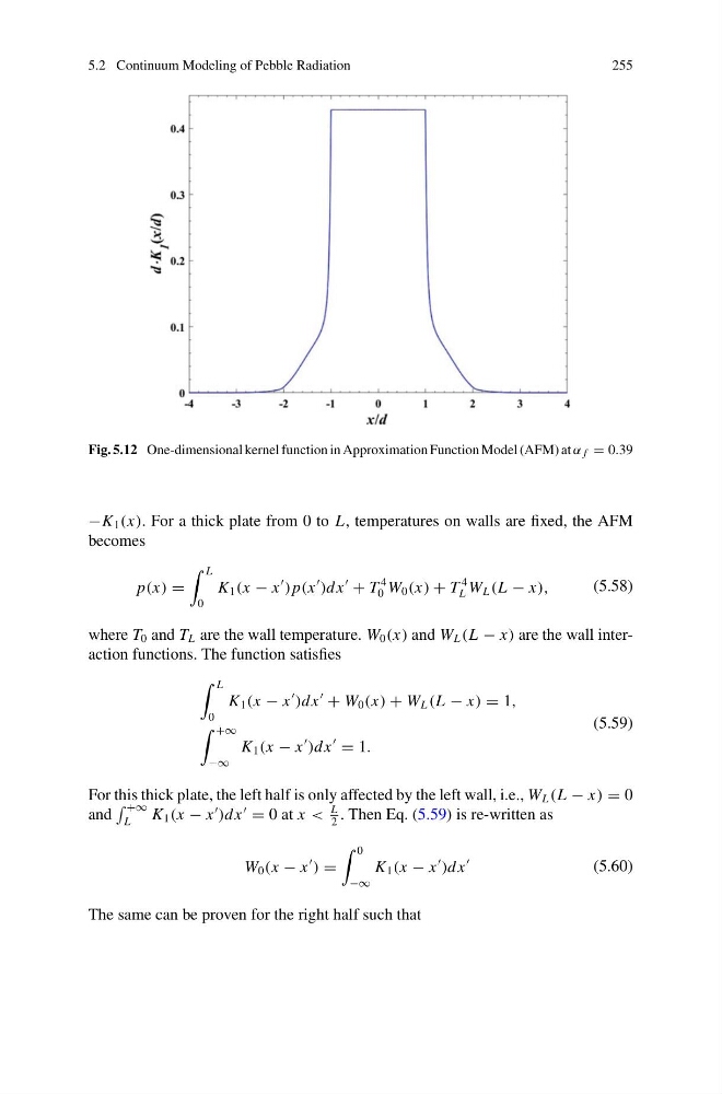
Fig. 5.12 One-dimensional kernel function in Approximation Function Model (AFM) at α f = 0.39
−K 1 (x). For a thick plate from 0 to L, temperatures on walls are fixed, the AFM
becomes
p(x) =
L
0
K 1 (x − x
) p(x
)dx
+ T
4
0 W 0 (x) + T
4
L W L (L − x),
(5.58)
where T 0 and T L are the wall temperature. W 0 (x) and W L (L − x) are the wall interaction functions. The function satisfies
L
0
K 1 (x − x
)dx
+ W 0 (x) + W L (L − x) = 1,
+∞
−∞
K 1 (x − x
)dx
= 1.
(5.59)
For this thick plate, the left half is only affected by the left wall, i.e., W L (L − x) = 0
and
+∞
L
K 1 (x − x
)dx
= 0 at x <
L
2
. Then Eq. (5.59) is re-written as
W 0 (x − x
) =
0
−∞
K 1 (x − x
)dx
(5.60)
The same can be proven for the right half such that
255
Fig. 5.12 One-dimensional kernel function in Approximation Function Model (AFM) at α f = 0.39
−K 1 (x). For a thick plate from 0 to L, temperatures on walls are fixed, the AFM
becomes
p(x) =
L
0
K 1 (x − x
) p(x
)dx
+ T
4
0 W 0 (x) + T
4
L W L (L − x),
(5.58)
where T 0 and T L are the wall temperature. W 0 (x) and W L (L − x) are the wall interaction functions. The function satisfies
L
0
K 1 (x − x
)dx
+ W 0 (x) + W L (L − x) = 1,
+∞
−∞
K 1 (x − x
)dx
= 1.
(5.59)
For this thick plate, the left half is only affected by the left wall, i.e., W L (L − x) = 0
and
+∞
L
K 1 (x − x
)dx
= 0 at x <
L
2
. Then Eq. (5.59) is re-written as
W 0 (x − x
) =
0
−∞
K 1 (x − x
)dx
(5.60)
The same can be proven for the right half such that