

226
4 Numerical Methods and Simulation for Pebble Flows
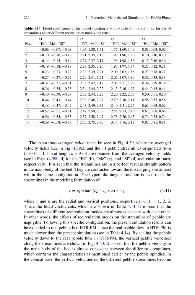
Table 4.14 Fitted coefficients of the model function: r = c 1 ∗ tanh(c 2 − c 3 ∗ h) + c 4 for the 14
streamlines under different recirculation modes and rates
c 1
c 2
c 3
c 4
Nos.
“Fa”, “Me”, “Sl”
“Fa”, “Me”, “Sl” “Fa”, “Me”, “Sl” “Fa”, “Me”, “Sl”
1
−0.06, −0.07, −0.08
1.95, 1.80, 1.51
1.77, 1.69, 1.49
0.03, 0.03, 0.02
2
−0.10, −0.10, −0.10
2.21, 2.35, 2.16
1.92, 1.96, 1.80
0.10, 0.10, 0.10
3
−0.14, −0.14, −0.14
2.27, 2.37, 2.17
1.96, 1.98, 1.80
0.15, 0.16, 0.16
4
−0.19, −0.18, −0.19
2.28, 2.35, 2.20
1.97, 1.97, 1.84
0.21, 0.22, 0.21
5
−0.23, −0.23, −0.23
2.30, 2.39, 2.21
2.00, 2.02, 1.86
0.27, 0.28, 0.27
6
−0.27, −0.27, −0.27
2.29, 2.41, 2.21
2.02, 2.07, 1.89
0.32, 0.33, 0.33
7
−0.31, −0.31, −0.31
2.32, 2.42, 2.19
2.07, 2.11, 1.90
0.38, 0.39, 0.39
8
−0.36, −0.35, −0.35
2.34, 2.44, 2.22
2.13, 2.16, 1.97
0.44, 0.45, 0.44
9
−0.40, −0.39, −0.39
2.36, 2.44, 2.26
2.20, 2.22, 2.05
0.50, 0.51, 0.50
10
−0.44, −0.43, −0.44
2.39, 2.46, 2.27
2.29, 2.30, 2.11
0.55, 0.57, 0.56
11
−0.48, −0.47, −0.47
2.43, 2.49, 2.34
2.40, 2.41, 2.26
0.61, 0.63, 0.62
12
−0.52, −0.51, −0.51
2.47, 2.50, 2.38
2.55, 2.53, 2.40
0.67, 0.68, 0.68
13
−0.56, −0.55, −0.55
2.57, 2.58, 2.47
2.78, 2.76, 2.63
0.74, 0.75, 0.74
14
−0.59, −0.58, −0.59
2.70, 2.75, 2.70
3.14, 3.16, 3.12
0.81, 0.81, 0.81
The mean time-averaged velocity can be seen in Fig. 4.39, where the averaged
velocity fields (see in Fig. 4.39a), and the 14 pebble streamlines originated from
(r = 0.1—1.4 m at height h = 9 m) are obtained from the averaged velocity fields
(see in Figs. (4.39b–d) for the “Fa” (b), “Me” (c), and “Sl” (d) recirculation rates,
respectively). It is seen that the streamlines are in a perfect vertical straight pattern
in the main body of the bed. They are contracted toward the discharging silo almost
within the same configuration. The hyperbolic tangent function is used to fit the
streamlines in the modeling formulation of
r = c 1 ∗ tanh(c 2 − c 3 ∗ h) + c 4 ,
(4.41)
where r and h are the radial and vertical positions, respectively. c i , (i = 1, 2, 3,
4) are the fitted coefficients, which are shown in Table 4.14. It is seen that the
streamlines of different recirculation modes are almost consistent with each other.
In other words, the effects of recirculation modes on the streamline of pebble are
negligible. Following this specific configuration, the present simulation results can
be extended to real pebble-bed HTR-PM, since the real pebble flow in HTR-PM is
much slower than the present simulation (see in Table 4.14). By scaling the pebble
velocity down to the real pebble flow in HTR-PM, the vertical pebble velocities
along the streamlines are shown in Fig. 4.40. It is seen that the pebble velocity in
the main body of the bed is almost consistent between the different streamlines,
which confirms the characteristics as mentioned earlier by the pebble spindles. In
the conical base, the vertical velocities on the different pebble streamlines become
4 Numerical Methods and Simulation for Pebble Flows
Table 4.14 Fitted coefficients of the model function: r = c 1 ∗ tanh(c 2 − c 3 ∗ h) + c 4 for the 14
streamlines under different recirculation modes and rates
c 1
c 2
c 3
c 4
Nos.
“Fa”, “Me”, “Sl”
“Fa”, “Me”, “Sl” “Fa”, “Me”, “Sl” “Fa”, “Me”, “Sl”
1
−0.06, −0.07, −0.08
1.95, 1.80, 1.51
1.77, 1.69, 1.49
0.03, 0.03, 0.02
2
−0.10, −0.10, −0.10
2.21, 2.35, 2.16
1.92, 1.96, 1.80
0.10, 0.10, 0.10
3
−0.14, −0.14, −0.14
2.27, 2.37, 2.17
1.96, 1.98, 1.80
0.15, 0.16, 0.16
4
−0.19, −0.18, −0.19
2.28, 2.35, 2.20
1.97, 1.97, 1.84
0.21, 0.22, 0.21
5
−0.23, −0.23, −0.23
2.30, 2.39, 2.21
2.00, 2.02, 1.86
0.27, 0.28, 0.27
6
−0.27, −0.27, −0.27
2.29, 2.41, 2.21
2.02, 2.07, 1.89
0.32, 0.33, 0.33
7
−0.31, −0.31, −0.31
2.32, 2.42, 2.19
2.07, 2.11, 1.90
0.38, 0.39, 0.39
8
−0.36, −0.35, −0.35
2.34, 2.44, 2.22
2.13, 2.16, 1.97
0.44, 0.45, 0.44
9
−0.40, −0.39, −0.39
2.36, 2.44, 2.26
2.20, 2.22, 2.05
0.50, 0.51, 0.50
10
−0.44, −0.43, −0.44
2.39, 2.46, 2.27
2.29, 2.30, 2.11
0.55, 0.57, 0.56
11
−0.48, −0.47, −0.47
2.43, 2.49, 2.34
2.40, 2.41, 2.26
0.61, 0.63, 0.62
12
−0.52, −0.51, −0.51
2.47, 2.50, 2.38
2.55, 2.53, 2.40
0.67, 0.68, 0.68
13
−0.56, −0.55, −0.55
2.57, 2.58, 2.47
2.78, 2.76, 2.63
0.74, 0.75, 0.74
14
−0.59, −0.58, −0.59
2.70, 2.75, 2.70
3.14, 3.16, 3.12
0.81, 0.81, 0.81
The mean time-averaged velocity can be seen in Fig. 4.39, where the averaged
velocity fields (see in Fig. 4.39a), and the 14 pebble streamlines originated from
(r = 0.1—1.4 m at height h = 9 m) are obtained from the averaged velocity fields
(see in Figs. (4.39b–d) for the “Fa” (b), “Me” (c), and “Sl” (d) recirculation rates,
respectively). It is seen that the streamlines are in a perfect vertical straight pattern
in the main body of the bed. They are contracted toward the discharging silo almost
within the same configuration. The hyperbolic tangent function is used to fit the
streamlines in the modeling formulation of
r = c 1 ∗ tanh(c 2 − c 3 ∗ h) + c 4 ,
(4.41)
where r and h are the radial and vertical positions, respectively. c i , (i = 1, 2, 3,
4) are the fitted coefficients, which are shown in Table 4.14. It is seen that the
streamlines of different recirculation modes are almost consistent with each other.
In other words, the effects of recirculation modes on the streamline of pebble are
negligible. Following this specific configuration, the present simulation results can
be extended to real pebble-bed HTR-PM, since the real pebble flow in HTR-PM is
much slower than the present simulation (see in Table 4.14). By scaling the pebble
velocity down to the real pebble flow in HTR-PM, the vertical pebble velocities
along the streamlines are shown in Fig. 4.40. It is seen that the pebble velocity in
the main body of the bed is almost consistent between the different streamlines,
which confirms the characteristics as mentioned earlier by the pebble spindles. In
the conical base, the vertical velocities on the different pebble streamlines become