

3.3 Effective Thermal Diffusivity and Conductivity
149
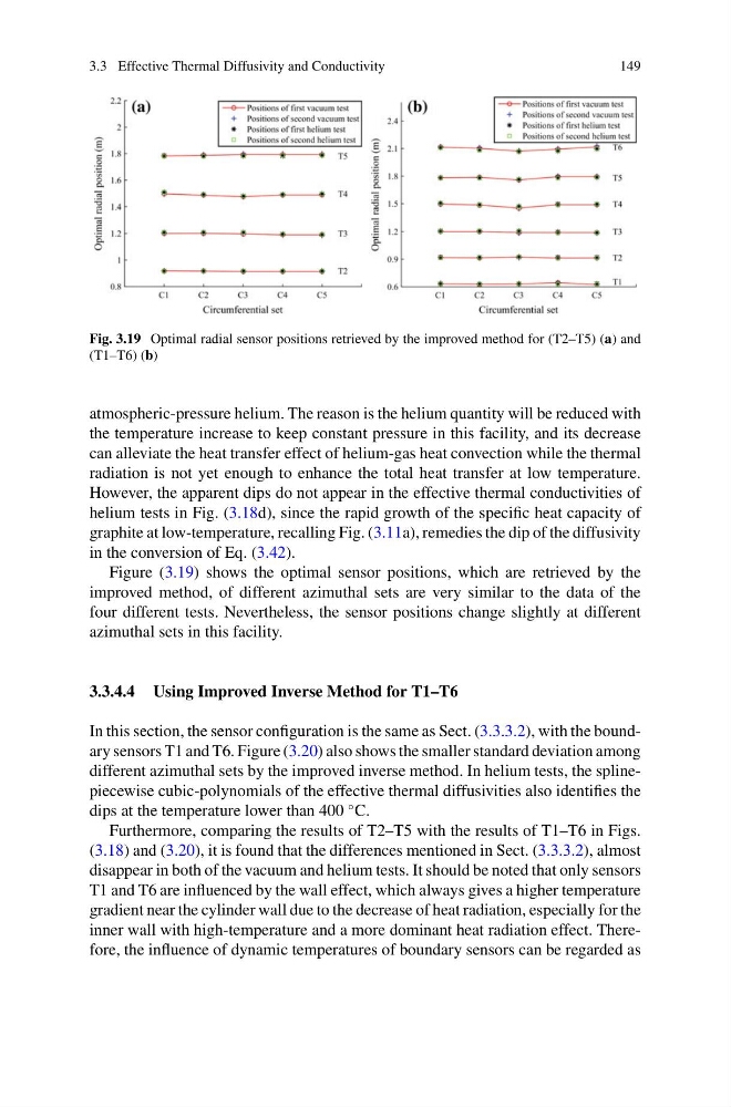
Fig. 3.19 Optimal radial sensor positions retrieved by the improved method for (T2–T5) (a) and
(T1–T6) (b)
atmospheric-pressure helium. The reason is the helium quantity will be reduced with
the temperature increase to keep constant pressure in this facility, and its decrease
can alleviate the heat transfer effect of helium-gas heat convection while the thermal
radiation is not yet enough to enhance the total heat transfer at low temperature.
However, the apparent dips do not appear in the effective thermal conductivities of
helium tests in Fig. (3.18d), since the rapid growth of the specific heat capacity of
graphite at low-temperature, recalling Fig. (3.11a), remedies the dip of the diffusivity
in the conversion of Eq. (3.42).
Figure (3.19) shows the optimal sensor positions, which are retrieved by the
improved method, of different azimuthal sets are very similar to the data of the
four different tests. Nevertheless, the sensor positions change slightly at different
azimuthal sets in this facility.
3.3.4.4 Using Improved Inverse Method for T1–T6
In this section, the sensor configuration is the same as Sect. (3.3.3.2), with the boundary sensors T1 and T6. Figure (3.20) also shows the smaller standard deviation among
different azimuthal sets by the improved inverse method. In helium tests, the splinepiecewise cubic-polynomials of the effective thermal diffusivities also identifies the
dips at the temperature lower than 400
◦ C.
Furthermore, comparing the results of T2–T5 with the results of T1–T6 in Figs.
(3.18) and (3.20), it is found that the differences mentioned in Sect. (3.3.3.2), almost
disappear in both of the vacuum and helium tests. It should be noted that only sensors
T1 and T6 are influenced by the wall effect, which always gives a higher temperature
gradient near the cylinder wall due to the decrease of heat radiation, especially for the
inner wall with high-temperature and a more dominant heat radiation effect. Therefore, the influence of dynamic temperatures of boundary sensors can be regarded as
149
Fig. 3.19 Optimal radial sensor positions retrieved by the improved method for (T2–T5) (a) and
(T1–T6) (b)
atmospheric-pressure helium. The reason is the helium quantity will be reduced with
the temperature increase to keep constant pressure in this facility, and its decrease
can alleviate the heat transfer effect of helium-gas heat convection while the thermal
radiation is not yet enough to enhance the total heat transfer at low temperature.
However, the apparent dips do not appear in the effective thermal conductivities of
helium tests in Fig. (3.18d), since the rapid growth of the specific heat capacity of
graphite at low-temperature, recalling Fig. (3.11a), remedies the dip of the diffusivity
in the conversion of Eq. (3.42).
Figure (3.19) shows the optimal sensor positions, which are retrieved by the
improved method, of different azimuthal sets are very similar to the data of the
four different tests. Nevertheless, the sensor positions change slightly at different
azimuthal sets in this facility.
3.3.4.4 Using Improved Inverse Method for T1–T6
In this section, the sensor configuration is the same as Sect. (3.3.3.2), with the boundary sensors T1 and T6. Figure (3.20) also shows the smaller standard deviation among
different azimuthal sets by the improved inverse method. In helium tests, the splinepiecewise cubic-polynomials of the effective thermal diffusivities also identifies the
dips at the temperature lower than 400
◦ C.
Furthermore, comparing the results of T2–T5 with the results of T1–T6 in Figs.
(3.18) and (3.20), it is found that the differences mentioned in Sect. (3.3.3.2), almost
disappear in both of the vacuum and helium tests. It should be noted that only sensors
T1 and T6 are influenced by the wall effect, which always gives a higher temperature
gradient near the cylinder wall due to the decrease of heat radiation, especially for the
inner wall with high-temperature and a more dominant heat radiation effect. Therefore, the influence of dynamic temperatures of boundary sensors can be regarded as