

142
3 Experiments in Pebble Bed Heat Transfer
to determine a proper initial value and avoid falling into inauthentic local minima
[24]. The iteration should stop when it meets the basic convergence criterion that S
only changes a little bit between two iterations.
3.3.3 Quadratic Polynomial Function Results
This section first presents and discusses the repeatable quadratic polynomial results
described by Eqs. (3.41) to (3.43), from the two vacuum tests and the two helium
tests. The quadratic polynomial diffusivity and its conductivity are calculated by
the aforementioned method in each azimuthal set, namely, C1–C5, to identify the
effects of thermocouple installation and random packing structure. Moreover, in
consideration of the variation of the packing structure near the inner and outer wall
[10], the boundary conditions are chosen as T2–T5 and T1–T6 to compare the wall
effect in results since T1 and T6 thermocouples are near the wall in this facility.
3.3.3.1 For T2–T5 Without Wall Effect
In this section, the boundary points are T2 and T5, and the compared middle points
included in P of Eqs. (3.11)–(3.12) are T3 and T4. The results of this section show
the diffusivity and conductivity of the bulk region of the pebble bed. The optimal quadratic polynomial effective thermal diffusivities are retrieved by the inverse
method through the recorded transient temperatures of first and second tests. Subsequently, the effective thermal conductivities are converted from diffusivities by Eqs.
(3.41) and (3.42).
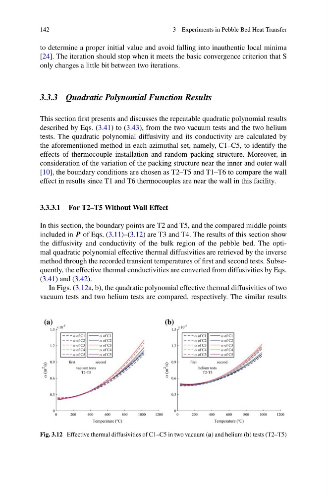
In Figs. (3.12a, b), the quadratic polynomial effective thermal diffusivities of two
vacuum tests and two helium tests are compared, respectively. The similar results
Fig. 3.12 Effective thermal diffusivities of C1–C5 in two vacuum (a) and helium (b) tests (T2–T5)
3 Experiments in Pebble Bed Heat Transfer
to determine a proper initial value and avoid falling into inauthentic local minima
[24]. The iteration should stop when it meets the basic convergence criterion that S
only changes a little bit between two iterations.
3.3.3 Quadratic Polynomial Function Results
This section first presents and discusses the repeatable quadratic polynomial results
described by Eqs. (3.41) to (3.43), from the two vacuum tests and the two helium
tests. The quadratic polynomial diffusivity and its conductivity are calculated by
the aforementioned method in each azimuthal set, namely, C1–C5, to identify the
effects of thermocouple installation and random packing structure. Moreover, in
consideration of the variation of the packing structure near the inner and outer wall
[10], the boundary conditions are chosen as T2–T5 and T1–T6 to compare the wall
effect in results since T1 and T6 thermocouples are near the wall in this facility.
3.3.3.1 For T2–T5 Without Wall Effect
In this section, the boundary points are T2 and T5, and the compared middle points
included in P of Eqs. (3.11)–(3.12) are T3 and T4. The results of this section show
the diffusivity and conductivity of the bulk region of the pebble bed. The optimal quadratic polynomial effective thermal diffusivities are retrieved by the inverse
method through the recorded transient temperatures of first and second tests. Subsequently, the effective thermal conductivities are converted from diffusivities by Eqs.
(3.41) and (3.42).
In Figs. (3.12a, b), the quadratic polynomial effective thermal diffusivities of two
vacuum tests and two helium tests are compared, respectively. The similar results
Fig. 3.12 Effective thermal diffusivities of C1–C5 in two vacuum (a) and helium (b) tests (T2–T5)