

4.2 Examples of χ (2) Tensor and Orientation
89
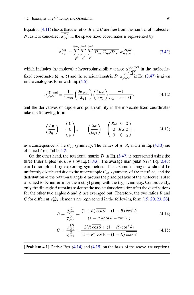
Equation (4.11) shows that the ratios B and C are free from the number of molecules
N , as it is cancelled. α
(2)
pqr in the space-fixed coordinates is represented by
α
(2)
pqr =
ξ ∼ζ
p
ξ ∼ζ
q
ξ ∼ζ
r
D pp D qq D rr α
(2),mol
p q r ,
(3.47)
which includes the molecular hyperpolarizability tensor α
(2),mol
p q r in the moleculefixed coordinates (ξ, η, ζ ) and the rotational matrix D. α
(2),mol
p q r in Eq. (3.47) is given
in the analogous form with Eq. (4.5),
α
(2),mol
p q r =
1
2mω
∂α p q
∂q 1
∂μ r
∂q 1
−1
ω 2 − ω + ii
,
(4.12)
and the derivatives of dipole and polarizability in the molecule-fixed coordinates
take the following form,
∂μ
∂q 1
=
⎛
⎝
0
0
μ
⎞
⎠ ,
∂α
∂q 1
=
⎛
⎝
Rα 0 0
0 Rα 0
0 0 α
⎞
⎠ ,
(4.13)
as a consequence of the C 3v symmetry. The values of μ, R, and α in Eq. (4.13) are
obtained from Table 4.2.
On the other hand, the rotational matrix D in Eq. (3.47) is represented using the
three Euler angles {φ, θ, ψ} by Eq. (3.43). The average manipulation in Eq. (3.47)
can be simplified by exploiting symmetries. The azimuthal angle φ should be
uniformly distributed due to the macroscopic C ∞ symmetry of the interface, and the
distribution of the rotational angle ψ around the principal axis of the molecule is also
assumed to be uniform for the methyl group with the C 3v symmetry. Consequently,
only the tilt angle θ remains to define the molecular orientation after the distributions
for the other two angles φ and ψ are averaged out. Therefore, the two ratios B and
C for different χ
(2)
pqr elements are represented in the following form [19, 20, 23, 28].
B =
χ
(2)
yyz
χ
(2)
yzy
=
(1 + R) cos θ − (1 − R) cos 3 θ
(1 − R)(cos θ − cos 3 θ)
(4.14)
C =
χ
(2)
zzz
χ
(2)
yyz
=
2{R cos θ + (1 − R) cos 3 θ }
(1 + R) cos θ − (1 − R) cos 3 θ
(4.15)
[Problem 4.1] Derive Eqs. (4.14) and (4.15) on the basis of the above assumptions.
89
Equation (4.11) shows that the ratios B and C are free from the number of molecules
N , as it is cancelled. α
(2)
pqr in the space-fixed coordinates is represented by
α
(2)
pqr =
ξ ∼ζ
p
ξ ∼ζ
q
ξ ∼ζ
r
D pp D qq D rr α
(2),mol
p q r ,
(3.47)
which includes the molecular hyperpolarizability tensor α
(2),mol
p q r in the moleculefixed coordinates (ξ, η, ζ ) and the rotational matrix D. α
(2),mol
p q r in Eq. (3.47) is given
in the analogous form with Eq. (4.5),
α
(2),mol
p q r =
1
2mω
∂α p q
∂q 1
∂μ r
∂q 1
−1
ω 2 − ω + ii
,
(4.12)
and the derivatives of dipole and polarizability in the molecule-fixed coordinates
take the following form,
∂μ
∂q 1
=
⎛
⎝
0
0
μ
⎞
⎠ ,
∂α
∂q 1
=
⎛
⎝
Rα 0 0
0 Rα 0
0 0 α
⎞
⎠ ,
(4.13)
as a consequence of the C 3v symmetry. The values of μ, R, and α in Eq. (4.13) are
obtained from Table 4.2.
On the other hand, the rotational matrix D in Eq. (3.47) is represented using the
three Euler angles {φ, θ, ψ} by Eq. (3.43). The average manipulation in Eq. (3.47)
can be simplified by exploiting symmetries. The azimuthal angle φ should be
uniformly distributed due to the macroscopic C ∞ symmetry of the interface, and the
distribution of the rotational angle ψ around the principal axis of the molecule is also
assumed to be uniform for the methyl group with the C 3v symmetry. Consequently,
only the tilt angle θ remains to define the molecular orientation after the distributions
for the other two angles φ and ψ are averaged out. Therefore, the two ratios B and
C for different χ
(2)
pqr elements are represented in the following form [19, 20, 23, 28].
B =
χ
(2)
yyz
χ
(2)
yzy
=
(1 + R) cos θ − (1 − R) cos 3 θ
(1 − R)(cos θ − cos 3 θ)
(4.14)
C =
χ
(2)
zzz
χ
(2)
yyz
=
2{R cos θ + (1 − R) cos 3 θ }
(1 + R) cos θ − (1 − R) cos 3 θ
(4.15)
[Problem 4.1] Derive Eqs. (4.14) and (4.15) on the basis of the above assumptions.