

86
4 Two Computational Schemes of χ (2)
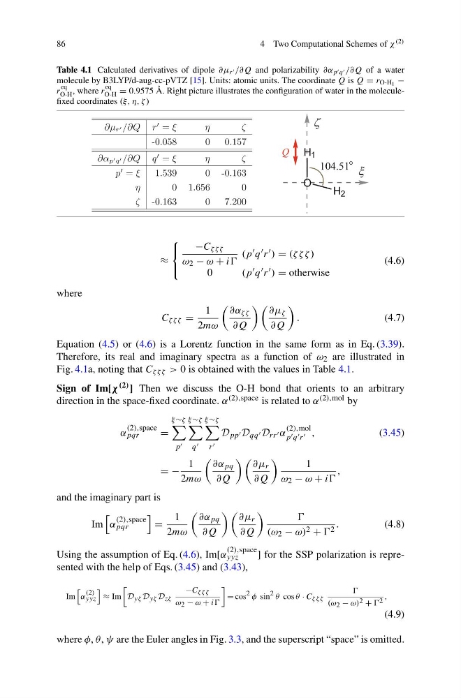
Table 4.1 Calculated derivatives of dipole ∂μ r /∂Q and polarizability ∂α p q /∂Q of a water
molecule by B3LYP/d-aug-cc-pVTZ [15]. Units: atomic units. The coordinate Q is Q = r O-H 1 −
r
eq
O-H , where r
eq
O-H = 0.9575 Å. Right picture illustrates the configuration of water in the moleculefixed coordinates (ξ, η, ζ )
H 1
O
H 2
104.51
Q
≈
⎧
⎨
⎩
−C ζ ζ ζ
ω 2 − ω + ii
(p q r ) = (ζ ζ ζ )
0
(p q r ) = otherwise
(4.6)
where
C ζ ζ ζ =
1
2mω
∂α ζ ζ
∂Q
∂μ ζ
∂Q
.
(4.7)
Equation (4.5) or (4.6) is a Lorentz function in the same form as in Eq. (3.39).
Therefore, its real and imaginary spectra as a function of ω 2 are illustrated in
Fig. 4.1a, noting that C ζ ζ ζ > 0 is obtained with the values in Table 4.1.
Sign of Im[χ (2) ] Then we discuss the O-H bond that orients to an arbitrary
direction in the space-fixed coordinate. α (2),space is related to α (2),mol by
α
(2),space
pqr
=
ξ ∼ζ
p
ξ ∼ζ
q
ξ ∼ζ
r
D pp D qq D rr α
(2),mol
p q r ,
(3.45)
= −
1
2mω
∂α pq
∂Q
∂μ r
∂Q
1
ω 2 − ω + ii
,
and the imaginary part is
Im
α
(2),space
pqr
=
1
2mω
∂α pq
∂Q
∂μ r
∂Q
(ω 2 − ω) 2 + 2 .
(4.8)
Using the assumption of Eq. (4.6), Im[α
(2),space
yyz
] for the SSP polarization is represented with the help of Eqs. (3.45) and (3.43),
Im
α
(2)
yyz
≈ Im
D yζ D yζ D zζ
−C ζ ζ ζ
ω 2 − ω + ii
= cos 2 φ sin 2 θ cos θ · C ζ ζ ζ
(ω 2 − ω) 2 + 2 ,
(4.9)
where φ, θ , ψ are the Euler angles in Fig. 3.3, and the superscript “space” is omitted.
4 Two Computational Schemes of χ (2)
Table 4.1 Calculated derivatives of dipole ∂μ r /∂Q and polarizability ∂α p q /∂Q of a water
molecule by B3LYP/d-aug-cc-pVTZ [15]. Units: atomic units. The coordinate Q is Q = r O-H 1 −
r
eq
O-H , where r
eq
O-H = 0.9575 Å. Right picture illustrates the configuration of water in the moleculefixed coordinates (ξ, η, ζ )
H 1
O
H 2
104.51
Q
≈
⎧
⎨
⎩
−C ζ ζ ζ
ω 2 − ω + ii
(p q r ) = (ζ ζ ζ )
0
(p q r ) = otherwise
(4.6)
where
C ζ ζ ζ =
1
2mω
∂α ζ ζ
∂Q
∂μ ζ
∂Q
.
(4.7)
Equation (4.5) or (4.6) is a Lorentz function in the same form as in Eq. (3.39).
Therefore, its real and imaginary spectra as a function of ω 2 are illustrated in
Fig. 4.1a, noting that C ζ ζ ζ > 0 is obtained with the values in Table 4.1.
Sign of Im[χ (2) ] Then we discuss the O-H bond that orients to an arbitrary
direction in the space-fixed coordinate. α (2),space is related to α (2),mol by
α
(2),space
pqr
=
ξ ∼ζ
p
ξ ∼ζ
q
ξ ∼ζ
r
D pp D qq D rr α
(2),mol
p q r ,
(3.45)
= −
1
2mω
∂α pq
∂Q
∂μ r
∂Q
1
ω 2 − ω + ii
,
and the imaginary part is
Im
α
(2),space
pqr
=
1
2mω
∂α pq
∂Q
∂μ r
∂Q
(ω 2 − ω) 2 + 2 .
(4.8)
Using the assumption of Eq. (4.6), Im[α
(2),space
yyz
] for the SSP polarization is represented with the help of Eqs. (3.45) and (3.43),
Im
α
(2)
yyz
≈ Im
D yζ D yζ D zζ
−C ζ ζ ζ
ω 2 − ω + ii
= cos 2 φ sin 2 θ cos θ · C ζ ζ ζ
(ω 2 − ω) 2 + 2 ,
(4.9)
where φ, θ , ψ are the Euler angles in Fig. 3.3, and the superscript “space” is omitted.