

4.2 Examples of χ (2) Tensor and Orientation
85
mg
mg
(a) C mg > 0
(b) C mg < 0
O
H
H
C
H
H
H
O
H
H
C
H
H
H
Water O-H
Methyl sym. C-H
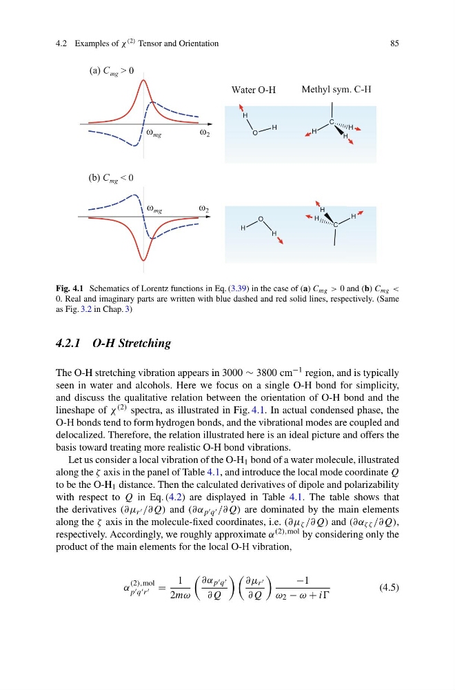
Fig. 4.1 Schematics of Lorentz functions in Eq. (3.39) in the case of (a) C mg > 0 and (b) C mg <
0. Real and imaginary parts are written with blue dashed and red solid lines, respectively. (Same
as Fig. 3.2 in Chap. 3)
4.2.1 O-H Stretching
The O-H stretching vibration appears in 3000 ∼ 3800 cm −1 region, and is typically
seen in water and alcohols. Here we focus on a single O-H bond for simplicity,
and discuss the qualitative relation between the orientation of O-H bond and the
lineshape of χ (2) spectra, as illustrated in Fig. 4.1. In actual condensed phase, the
O-H bonds tend to form hydrogen bonds, and the vibrational modes are coupled and
delocalized. Therefore, the relation illustrated here is an ideal picture and offers the
basis toward treating more realistic O-H bond vibrations.
Let us consider a local vibration of the O-H 1 bond of a water molecule, illustrated
along the ζ axis in the panel of Table 4.1, and introduce the local mode coordinate Q
to be the O-H 1 distance. Then the calculated derivatives of dipole and polarizability
with respect to Q in Eq. (4.2) are displayed in Table 4.1. The table shows that
the derivatives (∂μ r /∂Q) and (∂α p q /∂Q) are dominated by the main elements
along the ζ axis in the molecule-fixed coordinates, i.e. (∂μ ζ /∂Q) and (∂α ζ ζ /∂Q),
respectively. Accordingly, we roughly approximate α (2),mol by considering only the
product of the main elements for the local O-H vibration,
α
(2),mol
p q r =
1
2mω
∂α p q
∂Q
∂μ r
∂Q
−1
ω 2 − ω + ii
(4.5)
85
mg
mg
(a) C mg > 0
(b) C mg < 0
O
H
H
C
H
H
H
O
H
H
C
H
H
H
Water O-H
Methyl sym. C-H
Fig. 4.1 Schematics of Lorentz functions in Eq. (3.39) in the case of (a) C mg > 0 and (b) C mg <
0. Real and imaginary parts are written with blue dashed and red solid lines, respectively. (Same
as Fig. 3.2 in Chap. 3)
4.2.1 O-H Stretching
The O-H stretching vibration appears in 3000 ∼ 3800 cm −1 region, and is typically
seen in water and alcohols. Here we focus on a single O-H bond for simplicity,
and discuss the qualitative relation between the orientation of O-H bond and the
lineshape of χ (2) spectra, as illustrated in Fig. 4.1. In actual condensed phase, the
O-H bonds tend to form hydrogen bonds, and the vibrational modes are coupled and
delocalized. Therefore, the relation illustrated here is an ideal picture and offers the
basis toward treating more realistic O-H bond vibrations.
Let us consider a local vibration of the O-H 1 bond of a water molecule, illustrated
along the ζ axis in the panel of Table 4.1, and introduce the local mode coordinate Q
to be the O-H 1 distance. Then the calculated derivatives of dipole and polarizability
with respect to Q in Eq. (4.2) are displayed in Table 4.1. The table shows that
the derivatives (∂μ r /∂Q) and (∂α p q /∂Q) are dominated by the main elements
along the ζ axis in the molecule-fixed coordinates, i.e. (∂μ ζ /∂Q) and (∂α ζ ζ /∂Q),
respectively. Accordingly, we roughly approximate α (2),mol by considering only the
product of the main elements for the local O-H vibration,
α
(2),mol
p q r =
1
2mω
∂α p q
∂Q
∂μ r
∂Q
−1
ω 2 − ω + ii
(4.5)