

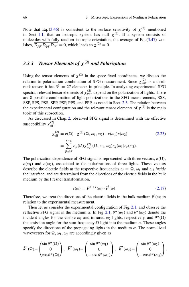
66
3 Microscopic Expressions of Nonlinear Polarization
Note that Eq. (3.46) is consistent to the surface sensitivity of χ (2) mentioned
in Sect. 1.1, that an isotropic system has null χ (2) . If a system consists of
molecules with fully random isotropic orientation, the average of Eq. (3.47) vanishes, D pp D qq D rr = 0, which leads to χ (2) = 0.
3.3.3 Tensor Elements of χ (2) and Polarization
Using the tensor elements of χ (2) in the space-fixed coordinates, we discuss the
relation to polarization combination of SFG measurement. Since χ
(2)
pqr is a thirdrank tensor, it has 3 3 = 27 elements in principle. In analyzing experimental SFG
spectra, relevant tensor elements of χ
(2)
pqr depend on the polarization of lights. There
are 8 possible combination of light polarizations in the SFG measurements, SSS,
SSP, SPS, PSS, SPP, PSP, PPS, and PPP, as noted in Sect. 2.3. The relation between
the experimental configuration and the relevant tensor elements of χ (2) is the main
topic of this subsection.
As discussed in Chap. 2, observed SFG signal is determined with the effective
susceptibility χ
(2)
eff ,
χ
(2)
eff = e(() · χ
(2) ((, ω 1 , ω 2 ) : e(ω 1 )e(ω 2 )
(2.23)
=
x∼z
p,q,r
e p (()χ
(2)
pqr ((, ω 1 , ω 2 )e q (ω 1 )e r (ω 2 ).
The polarization dependence of SFG signal is represented with three vectors, e((),
e(ω 1 ) and e(ω 2 ), associated to the polarizations of three lights. These vectors
describe the electric fields at the respective frequencies ω = , ω 1 and ω 2 inside
the interface, and are determined from the directions of the electric fields in the bulk
medium by the Fresnel transformation,
e(ω) = F
i→j (ω) · ˆ
e
i (ω).
(2.17)
Therefore, we treat the directions of the electric fields in the bulk medium ˆ
e
i (ω) in
relation to the experimental measurement.
Then let us consider the experimental configuration of Fig. 2.1, and observe the
reflective SFG signal in the medium α. In Fig. 2.1, θ α (ω 1 ) and θ α (ω 2 ) denote the
incident angles for the visible ω 1 and infrared ω 2 lights, respectively, and θ α (()
the emission angle for the sum-frequency light into the medium α. These angles
specify the directions of the propagating lights in the medium α. The normalized
wavevectors for , ω 1 , ω 2 are accordingly given as
ˆ
k
α
(()=
⎛
⎝
sin θ α (()
0
cos θ α (()
⎞
⎠ , ˆ
k
α
(ω 1 )=
⎛
⎝
sin θ α (ω 1 )
0
− cos θ α (ω 1 )
⎞
⎠ , ˆ
k
α
(ω 2 )=
⎛
⎝
sin θ α (ω 2 )
0
− cos θ α (ω 2 )
⎞
⎠ .
3 Microscopic Expressions of Nonlinear Polarization
Note that Eq. (3.46) is consistent to the surface sensitivity of χ (2) mentioned
in Sect. 1.1, that an isotropic system has null χ (2) . If a system consists of
molecules with fully random isotropic orientation, the average of Eq. (3.47) vanishes, D pp D qq D rr = 0, which leads to χ (2) = 0.
3.3.3 Tensor Elements of χ (2) and Polarization
Using the tensor elements of χ (2) in the space-fixed coordinates, we discuss the
relation to polarization combination of SFG measurement. Since χ
(2)
pqr is a thirdrank tensor, it has 3 3 = 27 elements in principle. In analyzing experimental SFG
spectra, relevant tensor elements of χ
(2)
pqr depend on the polarization of lights. There
are 8 possible combination of light polarizations in the SFG measurements, SSS,
SSP, SPS, PSS, SPP, PSP, PPS, and PPP, as noted in Sect. 2.3. The relation between
the experimental configuration and the relevant tensor elements of χ (2) is the main
topic of this subsection.
As discussed in Chap. 2, observed SFG signal is determined with the effective
susceptibility χ
(2)
eff ,
χ
(2)
eff = e(() · χ
(2) ((, ω 1 , ω 2 ) : e(ω 1 )e(ω 2 )
(2.23)
=
x∼z
p,q,r
e p (()χ
(2)
pqr ((, ω 1 , ω 2 )e q (ω 1 )e r (ω 2 ).
The polarization dependence of SFG signal is represented with three vectors, e((),
e(ω 1 ) and e(ω 2 ), associated to the polarizations of three lights. These vectors
describe the electric fields at the respective frequencies ω = , ω 1 and ω 2 inside
the interface, and are determined from the directions of the electric fields in the bulk
medium by the Fresnel transformation,
e(ω) = F
i→j (ω) · ˆ
e
i (ω).
(2.17)
Therefore, we treat the directions of the electric fields in the bulk medium ˆ
e
i (ω) in
relation to the experimental measurement.
Then let us consider the experimental configuration of Fig. 2.1, and observe the
reflective SFG signal in the medium α. In Fig. 2.1, θ α (ω 1 ) and θ α (ω 2 ) denote the
incident angles for the visible ω 1 and infrared ω 2 lights, respectively, and θ α (()
the emission angle for the sum-frequency light into the medium α. These angles
specify the directions of the propagating lights in the medium α. The normalized
wavevectors for , ω 1 , ω 2 are accordingly given as
ˆ
k
α
(()=
⎛
⎝
sin θ α (()
0
cos θ α (()
⎞
⎠ , ˆ
k
α
(ω 1 )=
⎛
⎝
sin θ α (ω 1 )
0
− cos θ α (ω 1 )
⎞
⎠ , ˆ
k
α
(ω 2 )=
⎛
⎝
sin θ α (ω 2 )
0
− cos θ α (ω 2 )
⎞
⎠ .