

3.3 Properties of χ (2)
61
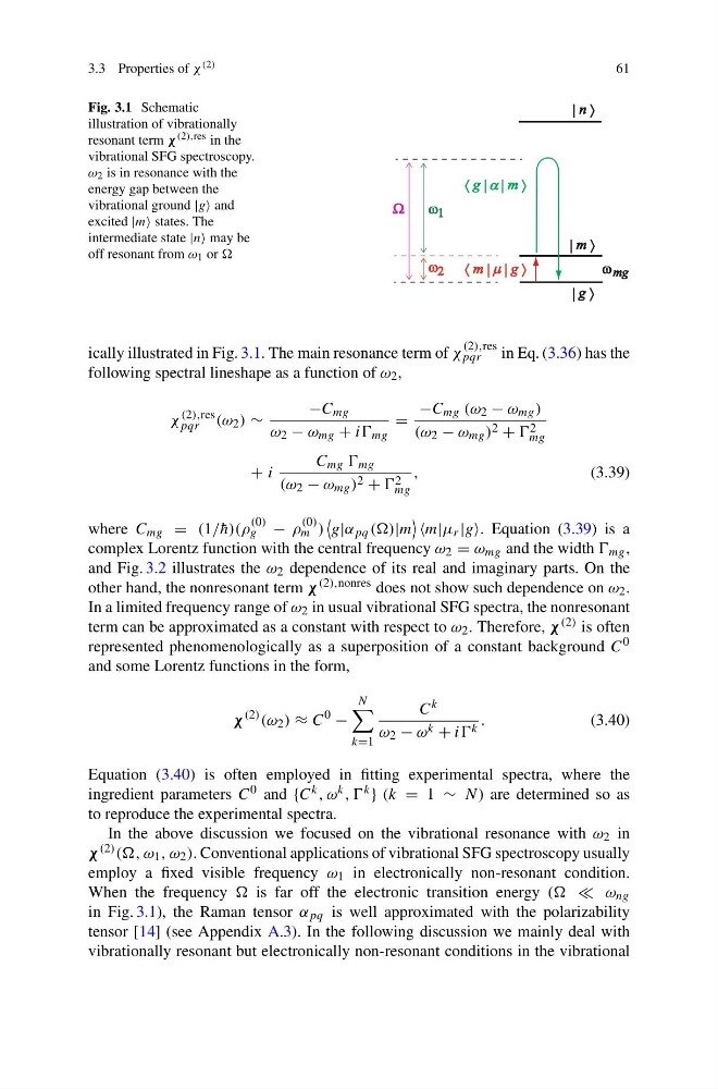
Fig. 3.1 Schematic
illustration of vibrationally
resonant term χ (2),res in the
vibrational SFG spectroscopy.
ω 2 is in resonance with the
energy gap between the
vibrational ground |g and
excited |m states. The
intermediate state |n may be
off resonant from ω 1 or
m
g
g
m
n
mg mg
g
m
2
1
ically illustrated in Fig. 3.1. The main resonance term of χ
(2),res
pqr
in Eq. (3.36) has the
following spectral lineshape as a function of ω 2 ,
χ
(2),res
pqr (ω 2 ) ∼
−C mg
ω 2 − ω mg + ii mg
=
−C mg (ω 2 − ω mg )
(ω 2 − ω mg ) 2 + 2
mg
+ i
C mg mg
(ω 2 − ω mg ) 2 + 2
mg
,
(3.39)
where C mg = (1/ ¯
h)(ρ
(0)
g − ρ
(0)
m )
g|α pq (()|m
m|μ r |g. Equation (3.39) is a
complex Lorentz function with the central frequency ω 2 = ω mg and the width mg ,
and Fig. 3.2 illustrates the ω 2 dependence of its real and imaginary parts. On the
other hand, the nonresonant term χ (2),nonres does not show such dependence on ω 2 .
In a limited frequency range of ω 2 in usual vibrational SFG spectra, the nonresonant
term can be approximated as a constant with respect to ω 2 . Therefore, χ (2) is often
represented phenomenologically as a superposition of a constant background C 0
and some Lorentz functions in the form,
χ
(2) (ω 2 ) ≈ C
0
−
N
k=1
C k
ω 2 − ω k + ii k .
(3.40)
Equation (3.40) is often employed in fitting experimental spectra, where the
ingredient parameters C 0 and {C k , ω k , , k } (k = 1 ∼ N ) are determined so as
to reproduce the experimental spectra.
In the above discussion we focused on the vibrational resonance with ω 2 in
χ (2) ((, ω 1 , ω 2 ). Conventional applications of vibrational SFG spectroscopy usually
employ a fixed visible frequency ω 1 in electronically non-resonant condition.
When the frequency is far off the electronic transition energy ( ω ng
in Fig. 3.1), the Raman tensor α pq is well approximated with the polarizability
tensor [14] (see Appendix A.3). In the following discussion we mainly deal with
vibrationally resonant but electronically non-resonant conditions in the vibrational
61
Fig. 3.1 Schematic
illustration of vibrationally
resonant term χ (2),res in the
vibrational SFG spectroscopy.
ω 2 is in resonance with the
energy gap between the
vibrational ground |g and
excited |m states. The
intermediate state |n may be
off resonant from ω 1 or
m
g
g
m
n
mg mg
g
m
2
1
ically illustrated in Fig. 3.1. The main resonance term of χ
(2),res
pqr
in Eq. (3.36) has the
following spectral lineshape as a function of ω 2 ,
χ
(2),res
pqr (ω 2 ) ∼
−C mg
ω 2 − ω mg + ii mg
=
−C mg (ω 2 − ω mg )
(ω 2 − ω mg ) 2 + 2
mg
+ i
C mg mg
(ω 2 − ω mg ) 2 + 2
mg
,
(3.39)
where C mg = (1/ ¯
h)(ρ
(0)
g − ρ
(0)
m )
g|α pq (()|m
m|μ r |g. Equation (3.39) is a
complex Lorentz function with the central frequency ω 2 = ω mg and the width mg ,
and Fig. 3.2 illustrates the ω 2 dependence of its real and imaginary parts. On the
other hand, the nonresonant term χ (2),nonres does not show such dependence on ω 2 .
In a limited frequency range of ω 2 in usual vibrational SFG spectra, the nonresonant
term can be approximated as a constant with respect to ω 2 . Therefore, χ (2) is often
represented phenomenologically as a superposition of a constant background C 0
and some Lorentz functions in the form,
χ
(2) (ω 2 ) ≈ C
0
−
N
k=1
C k
ω 2 − ω k + ii k .
(3.40)
Equation (3.40) is often employed in fitting experimental spectra, where the
ingredient parameters C 0 and {C k , ω k , , k } (k = 1 ∼ N ) are determined so as
to reproduce the experimental spectra.
In the above discussion we focused on the vibrational resonance with ω 2 in
χ (2) ((, ω 1 , ω 2 ). Conventional applications of vibrational SFG spectroscopy usually
employ a fixed visible frequency ω 1 in electronically non-resonant condition.
When the frequency is far off the electronic transition energy ( ω ng
in Fig. 3.1), the Raman tensor α pq is well approximated with the polarizability
tensor [14] (see Appendix A.3). In the following discussion we mainly deal with
vibrationally resonant but electronically non-resonant conditions in the vibrational