

A.1 Singularity of Source Polarization
35
D z
L
2
l
2
− D z
−
L
2
l
2
+
L/2
−L/2
dz
∂D x
∂x
+
∂D y
∂y
l
2
= −4π
L/2
−L/2
dz
∂P
(2)
x
∂x
+
∂P
(2)
y
∂y
l
2
= −4πl
2 L
∂
∂x
P S
x
L
+
∂
∂y
P S
y
L
= −4πl
2
∂P S
x
∂x
+
∂P S
y
∂y
.
(2.53)
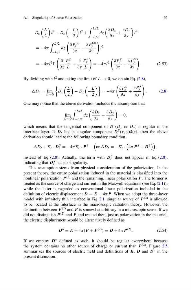
By dividing with l 2 and taking the limit of L → 0, we obtain Eq. (2.8),
D z = lim
L→0
D z
L
2
− D z
−
L
2
= −4π
∂P S
x
∂x
+
∂P S
y
∂y
.
(2.8)
One may notice that the above derivation includes the assumption that
lim
L→0
L/2
−L/2
dz
∂D x
∂x
+
∂D y
∂y
= 0,
which means that the tangential component of D (D x or D y ) is regular in the
interface layer. If D t had a singular component D S
t (x, y)δ(z), then the above
derivation should lead to the following boundary condition,
D z + ∇ t · D
S
t = −4π ∇ t · P
S
or D z = −∇ t ·
4π P
S
+ D
S
t
,
instead of Eq. (2.8). Actually, the term with D S
t does not appear in Eq. (2.8),
indicating that D S
t has no singularity.
This assumption stems from physical consideration of the polarization. In the
present theory, the entire polarization induced in the material is classified into the
nonlinear polarization P (2) and the remaining, linear polarization P . The former is
treated as the source of charge and current in the Maxwell equations (see Eq. (2.1)),
while the latter is regarded as conventional linear polarization included in the
definition of electric displacement D = E + 4π P . When we adopt the three-layer
model with infinitely thin interface in Fig. 2.1, singular source of P (2) is allowed
to be located at the interface in the macroscopic radiation theory. However, the
distinction between P (2) and P is somewhat arbitrary in a microscopic sense. If we
did not distinguish P (2) and P and treated them just as polarization in the material,
the electric displacement would be alternatively defined as
D
◦
= E + 4π(P + P
(2) ) = D + 4π P
(2) .
(2.54)
If we employ D ◦ defined as such, it should be regular everywhere because
the system contains no other source of charge or current than P (2) . Figure 2.5
summarizes the sources of electric field and definitions of E, D and D ◦ in the
present discussion.
35
D z
L
2
l
2
− D z
−
L
2
l
2
+
L/2
−L/2
dz
∂D x
∂x
+
∂D y
∂y
l
2
= −4π
L/2
−L/2
dz
∂P
(2)
x
∂x
+
∂P
(2)
y
∂y
l
2
= −4πl
2 L
∂
∂x
P S
x
L
+
∂
∂y
P S
y
L
= −4πl
2
∂P S
x
∂x
+
∂P S
y
∂y
.
(2.53)
By dividing with l 2 and taking the limit of L → 0, we obtain Eq. (2.8),
D z = lim
L→0
D z
L
2
− D z
−
L
2
= −4π
∂P S
x
∂x
+
∂P S
y
∂y
.
(2.8)
One may notice that the above derivation includes the assumption that
lim
L→0
L/2
−L/2
dz
∂D x
∂x
+
∂D y
∂y
= 0,
which means that the tangential component of D (D x or D y ) is regular in the
interface layer. If D t had a singular component D S
t (x, y)δ(z), then the above
derivation should lead to the following boundary condition,
D z + ∇ t · D
S
t = −4π ∇ t · P
S
or D z = −∇ t ·
4π P
S
+ D
S
t
,
instead of Eq. (2.8). Actually, the term with D S
t does not appear in Eq. (2.8),
indicating that D S
t has no singularity.
This assumption stems from physical consideration of the polarization. In the
present theory, the entire polarization induced in the material is classified into the
nonlinear polarization P (2) and the remaining, linear polarization P . The former is
treated as the source of charge and current in the Maxwell equations (see Eq. (2.1)),
while the latter is regarded as conventional linear polarization included in the
definition of electric displacement D = E + 4π P . When we adopt the three-layer
model with infinitely thin interface in Fig. 2.1, singular source of P (2) is allowed
to be located at the interface in the macroscopic radiation theory. However, the
distinction between P (2) and P is somewhat arbitrary in a microscopic sense. If we
did not distinguish P (2) and P and treated them just as polarization in the material,
the electric displacement would be alternatively defined as
D
◦
= E + 4π(P + P
(2) ) = D + 4π P
(2) .
(2.54)
If we employ D ◦ defined as such, it should be regular everywhere because
the system contains no other source of charge or current than P (2) . Figure 2.5
summarizes the sources of electric field and definitions of E, D and D ◦ in the
present discussion.