

7.3 Microscopic Formulas of Quadrupolar Susceptibilities
181
α
D0,res
pqr ((, ω 1 , ω 2 ) =
i
¯
h
∞
0
dt α pq ((, t)μ r − μ r α pq ((, t) exp(iω 2 t),
(7.101)
α
D1,res
pqrs ((, ω 1 , ω 2 ) =
i
¯
h
∞
0
dt β
psq (ω 1 , t)μ r − μ r β
psq (ω 1 , t) exp(iω 2 t),
(7.102)
α
D2,res
pqrs ((, ω 1 , ω 2 ) =
i
¯
h
∞
0
dt α pq ((, t)q sr (ω 2 ) − q sr (ω 2 )α pq ((, t) exp(iω 2 t),
(7.103)
α
Q,res
pqrs ((, ω 1 , ω 2 ) =
i
¯
h
∞
0
dt β spq ((, t)μ r − μ r β spq ((, t) exp(iω 2 t).
(7.104)
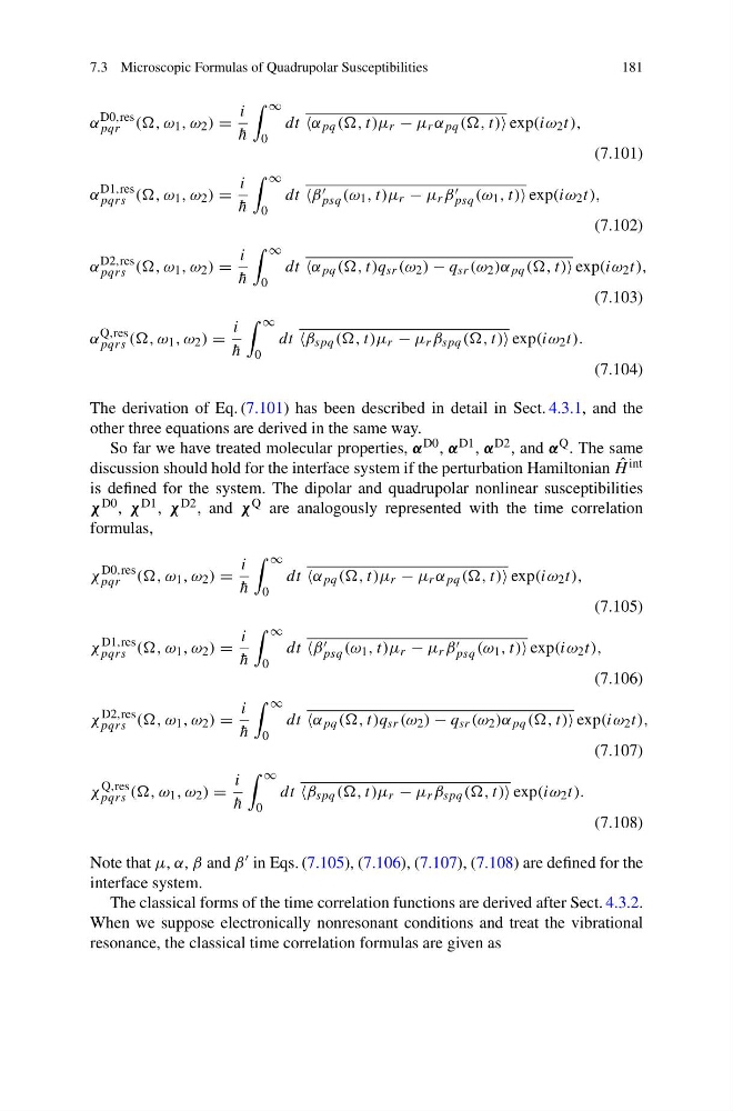
The derivation of Eq. (7.101) has been described in detail in Sect. 4.3.1, and the
other three equations are derived in the same way.
So far we have treated molecular properties, α D0 , α D1 , α D2 , and α Q . The same
discussion should hold for the interface system if the perturbation Hamiltonian ˆ
H int
is defined for the system. The dipolar and quadrupolar nonlinear susceptibilities
χ D0 , χ D1 , χ D2 , and χ Q are analogously represented with the time correlation
formulas,
χ
D0,res
pqr ((, ω 1 , ω 2 ) =
i
¯
h
∞
0
dt α pq ((, t)μ r − μ r α pq ((, t) exp(iω 2 t),
(7.105)
χ
D1,res
pqrs ((, ω 1 , ω 2 ) =
i
¯
h
∞
0
dt β
psq (ω 1 , t)μ r − μ r β
psq (ω 1 , t) exp(iω 2 t),
(7.106)
χ
D2,res
pqrs ((, ω 1 , ω 2 ) =
i
¯
h
∞
0
dt α pq ((, t)q sr (ω 2 ) − q sr (ω 2 )α pq ((, t) exp(iω 2 t),
(7.107)
χ
Q,res
pqrs ((, ω 1 , ω 2 ) =
i
¯
h
∞
0
dt β spq ((, t)μ r − μ r β spq ((, t) exp(iω 2 t).
(7.108)
Note that μ, α, β and β in Eqs. (7.105), (7.106), (7.107), (7.108) are defined for the
interface system.
The classical forms of the time correlation functions are derived after Sect. 4.3.2.
When we suppose electronically nonresonant conditions and treat the vibrational
resonance, the classical time correlation formulas are given as
181
α
D0,res
pqr ((, ω 1 , ω 2 ) =
i
¯
h
∞
0
dt α pq ((, t)μ r − μ r α pq ((, t) exp(iω 2 t),
(7.101)
α
D1,res
pqrs ((, ω 1 , ω 2 ) =
i
¯
h
∞
0
dt β
psq (ω 1 , t)μ r − μ r β
psq (ω 1 , t) exp(iω 2 t),
(7.102)
α
D2,res
pqrs ((, ω 1 , ω 2 ) =
i
¯
h
∞
0
dt α pq ((, t)q sr (ω 2 ) − q sr (ω 2 )α pq ((, t) exp(iω 2 t),
(7.103)
α
Q,res
pqrs ((, ω 1 , ω 2 ) =
i
¯
h
∞
0
dt β spq ((, t)μ r − μ r β spq ((, t) exp(iω 2 t).
(7.104)
The derivation of Eq. (7.101) has been described in detail in Sect. 4.3.1, and the
other three equations are derived in the same way.
So far we have treated molecular properties, α D0 , α D1 , α D2 , and α Q . The same
discussion should hold for the interface system if the perturbation Hamiltonian ˆ
H int
is defined for the system. The dipolar and quadrupolar nonlinear susceptibilities
χ D0 , χ D1 , χ D2 , and χ Q are analogously represented with the time correlation
formulas,
χ
D0,res
pqr ((, ω 1 , ω 2 ) =
i
¯
h
∞
0
dt α pq ((, t)μ r − μ r α pq ((, t) exp(iω 2 t),
(7.105)
χ
D1,res
pqrs ((, ω 1 , ω 2 ) =
i
¯
h
∞
0
dt β
psq (ω 1 , t)μ r − μ r β
psq (ω 1 , t) exp(iω 2 t),
(7.106)
χ
D2,res
pqrs ((, ω 1 , ω 2 ) =
i
¯
h
∞
0
dt α pq ((, t)q sr (ω 2 ) − q sr (ω 2 )α pq ((, t) exp(iω 2 t),
(7.107)
χ
Q,res
pqrs ((, ω 1 , ω 2 ) =
i
¯
h
∞
0
dt β spq ((, t)μ r − μ r β spq ((, t) exp(iω 2 t).
(7.108)
Note that μ, α, β and β in Eqs. (7.105), (7.106), (7.107), (7.108) are defined for the
interface system.
The classical forms of the time correlation functions are derived after Sect. 4.3.2.
When we suppose electronically nonresonant conditions and treat the vibrational
resonance, the classical time correlation formulas are given as