

7.2 Extended Nonlinear Susceptibility
171
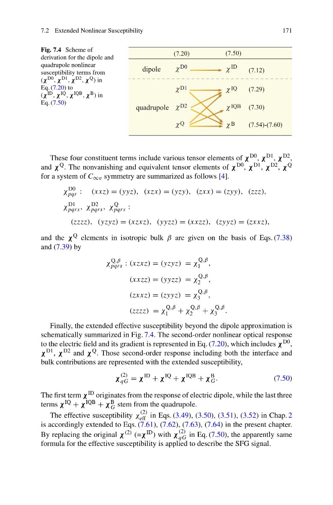
Fig. 7.4 Scheme of
derivation for the dipole and
quadrupole nonlinear
susceptibility terms from
(χ D0 , χ D1 , χ D2 , χ Q ) in
Eq. (7.20) to
(χ ID , χ IQ , χ IQB , χ B ) in
Eq. (7.50)
dipole
quadrupole
Q
D2
D1
D0
B
IQB
IQ
ID
(7.20)
(7.50)
(7.12)
(7.29)
(7.30)
(7.54)-(7.60)
These four constituent terms include various tensor elements of χ D0 , χ D1 , χ D2 ,
and χ Q . The nonvanishing and equivalent tensor elements of χ D0 , χ D1 , χ D2 , χ Q
for a system of C ∞v symmetry are summarized as follows [4].
χ
D0
pqr : (xxz) = (yyz), (xzx) = (yzy), (zxx) = (zyy), (zzz),
χ
D1
pqrs , χ
D2
pqrs , χ
Q
pqrs :
(zzzz), (yzyz) = (xzxz), (yyzz) = (xxzz), (zyyz) = (zxxz),
and the χ Q elements in isotropic bulk β are given on the basis of Eqs. (7.38)
and (7.39) by
χ
Q,β
pqrs : (xzxz) = (yzyz) = χ
Q,β
1 ,
(xxzz) = (yyzz) = χ
Q,β
2 ,
(zxxz) = (zyyz) = χ
Q,β
3 ,
(zzzz) = χ
Q,β
1
+ χ
Q,β
2
+ χ
Q,β
3 .
Finally, the extended effective susceptibility beyond the dipole approximation is
schematically summarized in Fig. 7.4. The second-order nonlinear optical response
to the electric field and its gradient is represented in Eq. (7.20), which includes χ D0 ,
χ D1 , χ D2 and χ Q . Those second-order response including both the interface and
bulk contributions are represented with the extended susceptibility,
χ
(2)
qG = χ
ID
+ χ
IQ
+ χ
IQB
+ χ
B
G .
(7.50)
The first term χ ID originates from the response of electric dipole, while the last three
terms χ IQ + χ IQB + χ B
G stem from the quadrupole.
The effective susceptibility χ
(2)
eff in Eqs. (3.49), (3.50), (3.51), (3.52) in Chap. 2
is accordingly extended to Eqs. (7.61), (7.62), (7.63), (7.64) in the present chapter.
By replacing the original χ (2) (=χ ID ) with χ
(2)
qG in Eq. (7.50), the apparently same
formula for the effective susceptibility is applied to describe the SFG signal.
171
Fig. 7.4 Scheme of
derivation for the dipole and
quadrupole nonlinear
susceptibility terms from
(χ D0 , χ D1 , χ D2 , χ Q ) in
Eq. (7.20) to
(χ ID , χ IQ , χ IQB , χ B ) in
Eq. (7.50)
dipole
quadrupole
Q
D2
D1
D0
B
IQB
IQ
ID
(7.20)
(7.50)
(7.12)
(7.29)
(7.30)
(7.54)-(7.60)
These four constituent terms include various tensor elements of χ D0 , χ D1 , χ D2 ,
and χ Q . The nonvanishing and equivalent tensor elements of χ D0 , χ D1 , χ D2 , χ Q
for a system of C ∞v symmetry are summarized as follows [4].
χ
D0
pqr : (xxz) = (yyz), (xzx) = (yzy), (zxx) = (zyy), (zzz),
χ
D1
pqrs , χ
D2
pqrs , χ
Q
pqrs :
(zzzz), (yzyz) = (xzxz), (yyzz) = (xxzz), (zyyz) = (zxxz),
and the χ Q elements in isotropic bulk β are given on the basis of Eqs. (7.38)
and (7.39) by
χ
Q,β
pqrs : (xzxz) = (yzyz) = χ
Q,β
1 ,
(xxzz) = (yyzz) = χ
Q,β
2 ,
(zxxz) = (zyyz) = χ
Q,β
3 ,
(zzzz) = χ
Q,β
1
+ χ
Q,β
2
+ χ
Q,β
3 .
Finally, the extended effective susceptibility beyond the dipole approximation is
schematically summarized in Fig. 7.4. The second-order nonlinear optical response
to the electric field and its gradient is represented in Eq. (7.20), which includes χ D0 ,
χ D1 , χ D2 and χ Q . Those second-order response including both the interface and
bulk contributions are represented with the extended susceptibility,
χ
(2)
qG = χ
ID
+ χ
IQ
+ χ
IQB
+ χ
B
G .
(7.50)
The first term χ ID originates from the response of electric dipole, while the last three
terms χ IQ + χ IQB + χ B
G stem from the quadrupole.
The effective susceptibility χ
(2)
eff in Eqs. (3.49), (3.50), (3.51), (3.52) in Chap. 2
is accordingly extended to Eqs. (7.61), (7.62), (7.63), (7.64) in the present chapter.
By replacing the original χ (2) (=χ ID ) with χ
(2)
qG in Eq. (7.50), the apparently same
formula for the effective susceptibility is applied to describe the SFG signal.