

7.1 Beyond the Three-Layer Model
155
where
P
(2) (z, ,) = f (z, ,)P
(2)
0 (z, ,)
= f (z, ,)
χ
D0 (z, ,, ω 1 , ω 2 ) :
f (z, ω 1 )L I (ω 1 )E
α
I (ω 1 )
f (z, ω 2 )L I (ω 2 )E
α
I (ω 2 )
.
(7.9)
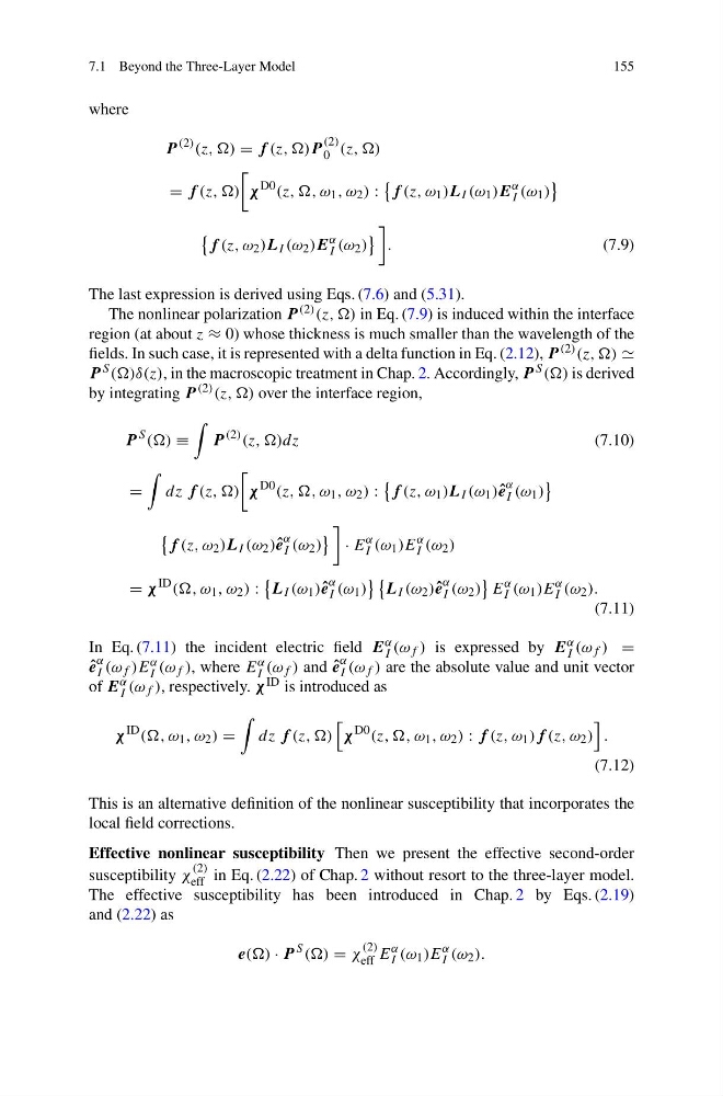
The last expression is derived using Eqs. (7.6) and (5.31).
The nonlinear polarization P (2) (z, ,) in Eq. (7.9) is induced within the interface
region (at about z ≈ 0) whose thickness is much smaller than the wavelength of the
fields. In such case, it is represented with a delta function in Eq. (2.12), P (2) (z, ,)
P S (()δ(z), in the macroscopic treatment in Chap. 2. Accordingly, P S (() is derived
by integrating P (2) (z, ,) over the interface region,
P
S (() ≡
P
(2) (z, ,)dz
(7.10)
=
dz f (z, ,)
χ
D0 (z, ,, ω 1 , ω 2 ) :
f (z, ω 1 )L I (ω 1 ) ˆ
e
α
I (ω 1 )
f (z, ω 2 )L I (ω 2 ) ˆ
e
α
I (ω 2 )
· E
α
I (ω 1 )E
α
I (ω 2 )
= χ
ID ((, ω 1 , ω 2 ) :
L I (ω 1 ) ˆ
e
α
I (ω 1 )
L I (ω 2 ) ˆ
e
α
I (ω 2 )
E
α
I (ω 1 )E
α
I (ω 2 ).
(7.11)
In Eq. (7.11) the incident electric field E α
I (ω f ) is expressed by E α
I (ω f ) =
ˆ
e
α
I (ω f )E α
I (ω f ), where E α
I (ω f ) and ˆ
e
α
I (ω f ) are the absolute value and unit vector
of E α
I (ω f ), respectively. χ ID is introduced as
χ
ID ((, ω 1 , ω 2 ) =
dz f (z, ,)
χ
D0 (z, ,, ω 1 , ω 2 ) : f (z, ω 1 )f (z, ω 2 )
.
(7.12)
This is an alternative definition of the nonlinear susceptibility that incorporates the
local field corrections.
Effective nonlinear susceptibility Then we present the effective second-order
susceptibility χ
(2)
eff in Eq. (2.22) of Chap. 2 without resort to the three-layer model.
The effective susceptibility has been introduced in Chap. 2 by Eqs. (2.19)
and (2.22) as
e(() · P
S (() = χ
(2)
eff E
α
I (ω 1 )E
α
I (ω 2 ).
155
where
P
(2) (z, ,) = f (z, ,)P
(2)
0 (z, ,)
= f (z, ,)
χ
D0 (z, ,, ω 1 , ω 2 ) :
f (z, ω 1 )L I (ω 1 )E
α
I (ω 1 )
f (z, ω 2 )L I (ω 2 )E
α
I (ω 2 )
.
(7.9)
The last expression is derived using Eqs. (7.6) and (5.31).
The nonlinear polarization P (2) (z, ,) in Eq. (7.9) is induced within the interface
region (at about z ≈ 0) whose thickness is much smaller than the wavelength of the
fields. In such case, it is represented with a delta function in Eq. (2.12), P (2) (z, ,)
P S (()δ(z), in the macroscopic treatment in Chap. 2. Accordingly, P S (() is derived
by integrating P (2) (z, ,) over the interface region,
P
S (() ≡
P
(2) (z, ,)dz
(7.10)
=
dz f (z, ,)
χ
D0 (z, ,, ω 1 , ω 2 ) :
f (z, ω 1 )L I (ω 1 ) ˆ
e
α
I (ω 1 )
f (z, ω 2 )L I (ω 2 ) ˆ
e
α
I (ω 2 )
· E
α
I (ω 1 )E
α
I (ω 2 )
= χ
ID ((, ω 1 , ω 2 ) :
L I (ω 1 ) ˆ
e
α
I (ω 1 )
L I (ω 2 ) ˆ
e
α
I (ω 2 )
E
α
I (ω 1 )E
α
I (ω 2 ).
(7.11)
In Eq. (7.11) the incident electric field E α
I (ω f ) is expressed by E α
I (ω f ) =
ˆ
e
α
I (ω f )E α
I (ω f ), where E α
I (ω f ) and ˆ
e
α
I (ω f ) are the absolute value and unit vector
of E α
I (ω f ), respectively. χ ID is introduced as
χ
ID ((, ω 1 , ω 2 ) =
dz f (z, ,)
χ
D0 (z, ,, ω 1 , ω 2 ) : f (z, ω 1 )f (z, ω 2 )
.
(7.12)
This is an alternative definition of the nonlinear susceptibility that incorporates the
local field corrections.
Effective nonlinear susceptibility Then we present the effective second-order
susceptibility χ
(2)
eff in Eq. (2.22) of Chap. 2 without resort to the three-layer model.
The effective susceptibility has been introduced in Chap. 2 by Eqs. (2.19)
and (2.22) as
e(() · P
S (() = χ
(2)
eff E
α
I (ω 1 )E
α
I (ω 2 ).