

2
1 Introduction
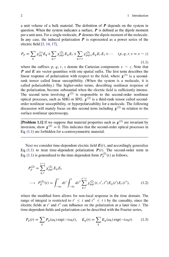
a unit volume of a bulk material. The definition of P depends on the system in
question. When the system indicates a surface, P is defined as the dipole moment
per a unit area. For a single molecule, P denotes the dipole moment of the molecule.
In any case, the induced polarization P is represented as a power series of the
electric field [3, 14, 17],
P p =
q
χ
(1)
pq E q +
q,r
χ
(2)
pqr E q E r +
q,r,s
χ
(3)
pqrs E q E r E s +· · · (p, q, r, s = x ∼ z)
(1.1)
where the suffixes p, q, r, s denote the Cartesian components x ∼ z. Note that
P and E are vector quantities with one spatial suffix. The first term describes the
linear response of polarization with respect to the field, where χ (1) is a secondrank tensor called linear susceptibility. (When the system is a molecule, it is
called polarizability.) The higher-order terms, describing nonlinear response of
the polarization, become substantial when the electric field is sufficiently intense.
The second term involving χ (2) is responsible to the second-order nonlinear
optical processes, such as SHG or SFG. χ (2) is a third-rank tensor called secondorder nonlinear susceptibility, or hyperpolarizability for a molecule. The following
discussion will mainly focus on this second term including χ (2) in relation to the
surface nonlinear spectroscopy.
[Problem 1.1] If we suppose that material properties such as χ (2) are invariant by
inversion, show χ (2) = 0. This indicates that the second-order optical processes in
Eq. (1.1) are forbidden for a centrosymmetric material.
Next we consider time-dependent electric field E(t), and accordingly generalize
Eq. (1.1) to treat time-dependent polarization P (t). The second-order term in
Eq. (1.1) is generalized to the time-dependent form P
(2)
p (t) as follows,
P
(2)
p =
x∼z
q,r
χ
(2)
pqr E q E r
−→ P
(2)
p (t) =
t
−∞
dt
t
−∞
dt
x∼z
q,r
χ
(2)
pqr (t, t
, t
)E q (t
)E r (t
),
(1.2)
where the modified form allows for non-local response in the time domain. The
range of integral is restricted to t ≤ t and t ≤ t t by the causality, since the
electric fields at t and t can influence on the polarization at a later time t. The
time-dependent fields and polarization can be described with the Fourier series,
P p (t) =
k
P p (ω k ) exp(−iω k t), E q (t) =
k
E q (ω k ) exp(−iω k t)
(1.3)
1 Introduction
a unit volume of a bulk material. The definition of P depends on the system in
question. When the system indicates a surface, P is defined as the dipole moment
per a unit area. For a single molecule, P denotes the dipole moment of the molecule.
In any case, the induced polarization P is represented as a power series of the
electric field [3, 14, 17],
P p =
q
χ
(1)
pq E q +
q,r
χ
(2)
pqr E q E r +
q,r,s
χ
(3)
pqrs E q E r E s +· · · (p, q, r, s = x ∼ z)
(1.1)
where the suffixes p, q, r, s denote the Cartesian components x ∼ z. Note that
P and E are vector quantities with one spatial suffix. The first term describes the
linear response of polarization with respect to the field, where χ (1) is a secondrank tensor called linear susceptibility. (When the system is a molecule, it is
called polarizability.) The higher-order terms, describing nonlinear response of
the polarization, become substantial when the electric field is sufficiently intense.
The second term involving χ (2) is responsible to the second-order nonlinear
optical processes, such as SHG or SFG. χ (2) is a third-rank tensor called secondorder nonlinear susceptibility, or hyperpolarizability for a molecule. The following
discussion will mainly focus on this second term including χ (2) in relation to the
surface nonlinear spectroscopy.
[Problem 1.1] If we suppose that material properties such as χ (2) are invariant by
inversion, show χ (2) = 0. This indicates that the second-order optical processes in
Eq. (1.1) are forbidden for a centrosymmetric material.
Next we consider time-dependent electric field E(t), and accordingly generalize
Eq. (1.1) to treat time-dependent polarization P (t). The second-order term in
Eq. (1.1) is generalized to the time-dependent form P
(2)
p (t) as follows,
P
(2)
p =
x∼z
q,r
χ
(2)
pqr E q E r
−→ P
(2)
p (t) =
t
−∞
dt
t
−∞
dt
x∼z
q,r
χ
(2)
pqr (t, t
, t
)E q (t
)E r (t
),
(1.2)
where the modified form allows for non-local response in the time domain. The
range of integral is restricted to t ≤ t and t ≤ t t by the causality, since the
electric fields at t and t can influence on the polarization at a later time t. The
time-dependent fields and polarization can be described with the Fourier series,
P p (t) =
k
P p (ω k ) exp(−iω k t), E q (t) =
k
E q (ω k ) exp(−iω k t)
(1.3)