

5.3 Interfacial Dielectric Constant ε
119
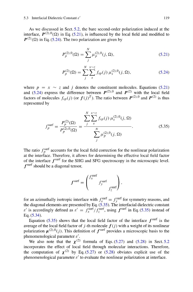
As we discussed in Sect. 5.2, the bare second-order polarization induced at the
interface, P (2),0 (() in Eq. (5.21), is influenced by the local field and modified to
P (2) (() in Eq. (5.24). The two polarization are given by
P
(2),0
p
(() =
N
j
μ
(2),0
p
(j, ,),
(5.21)
P
(2)
p (() =
N
j
x∼z
s
f sp (j ) μ
(2),0
s
(j, ,),
(5.24)
where p = x ∼ z and j denotes the constituent molecules. Equations (5.21)
and (5.24) express the difference between P (2),0 and P (2) with the local field
factors of molecules f sp (j ) (or f (j ) T ). The ratio between P (2),0 and P (2) is thus
represented by
f
surf
p
=
P
(2)
p (()
P
(2),0
p
(()
=
N
j
x∼z
s
f sp (j ) μ
(2),0
s
(j, ,)
N
j
μ
(2),0
p
(j, ,)
.
(5.35)
The ratio f surf
p
accounts for the local field correction for the nonlinear polarization
at the interface. Therefore, it allows for determining the effective local field factor
of the interface f
surf for the SHG and SFG spectroscopy in the microscopic level.
f
surf should be a diagonal tensor,
f
surf
=
⎛
⎝
f surf
x
f surf
y
f surf
z
⎞
⎠ ,
for an azimuthally isotropic interface with f surf
x
= f surf
y
for symmetry reasons, and
the diagonal elements are presented by Eq. (5.35). The interfacial dielectric constant
ε is accordingly defined as ε = f surf
x /f surf
z , using f
surf in Eq. (5.35) instead of
Eq. (5.34).
Equation (5.35) shows that the local field factor of the interface f
surf is the
average of the local field factor of j -th molecule f (j ) with a weight of its nonlinear
polarization μ (2),0 (j ). This definition of f
surf provides a microscopic basis to the
phenomenological parameter ε .
We also note that the χ (2) formula of Eqs. (5.27) and (5.28) in Sect. 5.2
incorporates the effect of local field through molecular interactions. Therefore,
the computation of χ (2) by Eq. (5.27) or (5.28) obviates explicit use of the
phenomenological parameter ε to evaluate the nonlinear polarization at interface.
119
As we discussed in Sect. 5.2, the bare second-order polarization induced at the
interface, P (2),0 (() in Eq. (5.21), is influenced by the local field and modified to
P (2) (() in Eq. (5.24). The two polarization are given by
P
(2),0
p
(() =
N
j
μ
(2),0
p
(j, ,),
(5.21)
P
(2)
p (() =
N
j
x∼z
s
f sp (j ) μ
(2),0
s
(j, ,),
(5.24)
where p = x ∼ z and j denotes the constituent molecules. Equations (5.21)
and (5.24) express the difference between P (2),0 and P (2) with the local field
factors of molecules f sp (j ) (or f (j ) T ). The ratio between P (2),0 and P (2) is thus
represented by
f
surf
p
=
P
(2)
p (()
P
(2),0
p
(()
=
N
j
x∼z
s
f sp (j ) μ
(2),0
s
(j, ,)
N
j
μ
(2),0
p
(j, ,)
.
(5.35)
The ratio f surf
p
accounts for the local field correction for the nonlinear polarization
at the interface. Therefore, it allows for determining the effective local field factor
of the interface f
surf for the SHG and SFG spectroscopy in the microscopic level.
f
surf should be a diagonal tensor,
f
surf
=
⎛
⎝
f surf
x
f surf
y
f surf
z
⎞
⎠ ,
for an azimuthally isotropic interface with f surf
x
= f surf
y
for symmetry reasons, and
the diagonal elements are presented by Eq. (5.35). The interfacial dielectric constant
ε is accordingly defined as ε = f surf
x /f surf
z , using f
surf in Eq. (5.35) instead of
Eq. (5.34).
Equation (5.35) shows that the local field factor of the interface f
surf is the
average of the local field factor of j -th molecule f (j ) with a weight of its nonlinear
polarization μ (2),0 (j ). This definition of f
surf provides a microscopic basis to the
phenomenological parameter ε .
We also note that the χ (2) formula of Eqs. (5.27) and (5.28) in Sect. 5.2
incorporates the effect of local field through molecular interactions. Therefore,
the computation of χ (2) by Eq. (5.27) or (5.28) obviates explicit use of the
phenomenological parameter ε to evaluate the nonlinear polarization at interface.