

118
5 Molecular Theory of Local Field
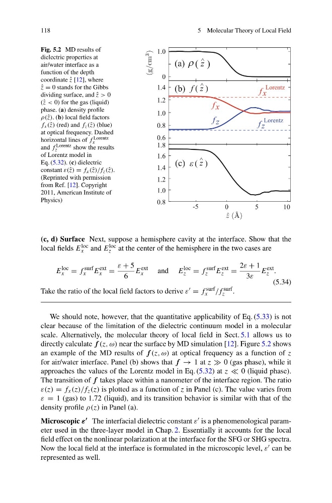
Fig. 5.2 MD results of
dielectric properties at
air/water interface as a
function of the depth
coordinate ˆ
z [12], where
ˆ
z = 0 stands for the Gibbs
dividing surface, and ˆ
z > 0
(ˆ z < 0) for the gas (liquid)
phase. (a) density profile
ρ(ˆ z). (b) local field factors
f x (ˆ z) (red) and f z (ˆ z) (blue)
at optical frequency. Dashed
horizontal lines of f Lorentz
x
and f Lorentz
z
show the results
of Lorentz model in
Eq. (5.32). (c) dielectric
constant ε(ˆ z) = f x (ˆ z)/f z (ˆ z).
(Reprinted with permission
from Ref. [12]. Copyright
2011, American Institute of
Physics)
f x
f z
f x
f z
Lorentz
Lorentz
-5
0
5
10
(a)
z
(b) f ( z )
(c)
z
0
1.0
1.4
1.2
1.0
0.8
0.6
1.4
1.2
1.0
0.8
1.6
1.8
^
^
^
(c, d) Surface Next, suppose a hemisphere cavity at the interface. Show that the
local fields E loc
x and E loc
z at the center of the hemisphere in the two cases are
E
loc
x = f
surf
x E
ext
x =
ε + 5
6
E
ext
x
and E
loc
z = f
surf
z E
ext
z =
2ε + 1
3ε
E
ext
z .
(5.34)
Take the ratio of the local field factors to derive ε = f surf
x /f surf
z .
We should note, however, that the quantitative applicability of Eq. (5.33) is not
clear because of the limitation of the dielectric continuum model in a molecular
scale. Alternatively, the molecular theory of local field in Sect. 5.1 allows us to
directly calculate f (z, ω) near the surface by MD simulation [12]. Figure 5.2 shows
an example of the MD results of f (z, ω) at optical frequency as a function of z
for air/water interface. Panel (b) shows that f → 1 at z 0 (gas phase), while it
approaches the values of the Lorentz model in Eq. (5.32) at z 0 (liquid phase).
The transition of f takes place within a nanometer of the interface region. The ratio
ε(z) = f x (z)/f z (z) is plotted as a function of z in Panel (c). The value varies from
ε = 1 (gas) to 1.72 (liquid), and its transition behavior is similar with that of the
density profile ρ(z) in Panel (a).
Microscopic ε The interfacial dielectric constant ε is a phenomenological parameter used in the three-layer model in Chap. 2. Essentially it accounts for the local
field effect on the nonlinear polarization at the interface for the SFG or SHG spectra.
Now the local field at the interface is formulated in the microscopic level, ε can be
represented as well.
5 Molecular Theory of Local Field
Fig. 5.2 MD results of
dielectric properties at
air/water interface as a
function of the depth
coordinate ˆ
z [12], where
ˆ
z = 0 stands for the Gibbs
dividing surface, and ˆ
z > 0
(ˆ z < 0) for the gas (liquid)
phase. (a) density profile
ρ(ˆ z). (b) local field factors
f x (ˆ z) (red) and f z (ˆ z) (blue)
at optical frequency. Dashed
horizontal lines of f Lorentz
x
and f Lorentz
z
show the results
of Lorentz model in
Eq. (5.32). (c) dielectric
constant ε(ˆ z) = f x (ˆ z)/f z (ˆ z).
(Reprinted with permission
from Ref. [12]. Copyright
2011, American Institute of
Physics)
f x
f z
f x
f z
Lorentz
Lorentz
-5
0
5
10
(a)
z
(b) f ( z )
(c)
z
0
1.0
1.4
1.2
1.0
0.8
0.6
1.4
1.2
1.0
0.8
1.6
1.8
^
^
^
(c, d) Surface Next, suppose a hemisphere cavity at the interface. Show that the
local fields E loc
x and E loc
z at the center of the hemisphere in the two cases are
E
loc
x = f
surf
x E
ext
x =
ε + 5
6
E
ext
x
and E
loc
z = f
surf
z E
ext
z =
2ε + 1
3ε
E
ext
z .
(5.34)
Take the ratio of the local field factors to derive ε = f surf
x /f surf
z .
We should note, however, that the quantitative applicability of Eq. (5.33) is not
clear because of the limitation of the dielectric continuum model in a molecular
scale. Alternatively, the molecular theory of local field in Sect. 5.1 allows us to
directly calculate f (z, ω) near the surface by MD simulation [12]. Figure 5.2 shows
an example of the MD results of f (z, ω) at optical frequency as a function of z
for air/water interface. Panel (b) shows that f → 1 at z 0 (gas phase), while it
approaches the values of the Lorentz model in Eq. (5.32) at z 0 (liquid phase).
The transition of f takes place within a nanometer of the interface region. The ratio
ε(z) = f x (z)/f z (z) is plotted as a function of z in Panel (c). The value varies from
ε = 1 (gas) to 1.72 (liquid), and its transition behavior is similar with that of the
density profile ρ(z) in Panel (a).
Microscopic ε The interfacial dielectric constant ε is a phenomenological parameter used in the three-layer model in Chap. 2. Essentially it accounts for the local
field effect on the nonlinear polarization at the interface for the SFG or SHG spectra.
Now the local field at the interface is formulated in the microscopic level, ε can be
represented as well.