

114
5 Molecular Theory of Local Field
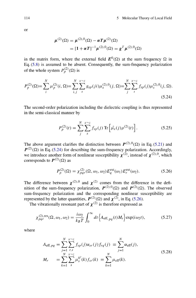
or
μ
(2) (() = μ
(2),0 (() − αT μ
(2) (()
= [1 + αT ]
−1 μ
(2),0 (() = g
T μ
(2),0 (()
in the matrix form, where the external field E 0 (() at the sum frequency in
Eq. (5.8) is assumed to be absent. Consequently, the sum-frequency polarization
of the whole system P
(2)
p (() is
P
(2)
p (()=
N
i
μ
(2)
p (i, ,)=
N
i,j
x∼z
s
g sp (j i)μ
(2),0
s
(j, ,)=
N
j
x∼z
s
f sp (j )μ
(2),0
s
(j, ,).
(5.24)
The second-order polarization including the dielectric coupling is thus represented
in the semi-classical manner by
P
(2)
p (t) =
N
j
x∼z
s
f sp (j ) Tr
ˆ
μ s (j )ρ
(2) (t)
.
(5.25)
The above argument clarifies the distinction between P (2),0 (() in Eq. (5.21) and
P (2) (() in Eq. (5.24) for describing the sum-frequency polarization. Accordingly,
we introduce another form of nonlinear susceptibility χ (2) , instead of χ (2),0 , which
corresponds to P (2) (() as
P
(2)
p (() = χ
(2)
pqr ((, ω 1 , ω 2 )E
ext
q (ω 1 )E
ext
r (ω 2 ).
(5.26)
The difference between χ (2),0 and χ (2) comes from the difference in the definition of the sum-frequency polarization, P (2),0 (() and P (2) ((). The observed
sum-frequency polarization and the corresponding nonlinear susceptibility are
represented by the latter quantities, P (2) (() and χ (2) , in Eq. (5.26).
The vibrationally resonant part of χ (2) is therefore expressed as
χ
(2),res
pqr ((, ω 1 , ω 2 ) =
iω 2
k B T
∞
0
dt
A eff, pq (t)M r
exp(iω 2 t),
(5.27)
where
A eff,pq =
N
j =1
x∼z
r,s
f sp (j )α sr (j )f rq (j ) ≡
N
j =1
α eff (j ),
M r
=
N
k=1
x∼z
s
μ
0
s
(k)f sr (k) ≡
N
k=1
μ eff (k).
(5.28)
5 Molecular Theory of Local Field
or
μ
(2) (() = μ
(2),0 (() − αT μ
(2) (()
= [1 + αT ]
−1 μ
(2),0 (() = g
T μ
(2),0 (()
in the matrix form, where the external field E 0 (() at the sum frequency in
Eq. (5.8) is assumed to be absent. Consequently, the sum-frequency polarization
of the whole system P
(2)
p (() is
P
(2)
p (()=
N
i
μ
(2)
p (i, ,)=
N
i,j
x∼z
s
g sp (j i)μ
(2),0
s
(j, ,)=
N
j
x∼z
s
f sp (j )μ
(2),0
s
(j, ,).
(5.24)
The second-order polarization including the dielectric coupling is thus represented
in the semi-classical manner by
P
(2)
p (t) =
N
j
x∼z
s
f sp (j ) Tr
ˆ
μ s (j )ρ
(2) (t)
.
(5.25)
The above argument clarifies the distinction between P (2),0 (() in Eq. (5.21) and
P (2) (() in Eq. (5.24) for describing the sum-frequency polarization. Accordingly,
we introduce another form of nonlinear susceptibility χ (2) , instead of χ (2),0 , which
corresponds to P (2) (() as
P
(2)
p (() = χ
(2)
pqr ((, ω 1 , ω 2 )E
ext
q (ω 1 )E
ext
r (ω 2 ).
(5.26)
The difference between χ (2),0 and χ (2) comes from the difference in the definition of the sum-frequency polarization, P (2),0 (() and P (2) ((). The observed
sum-frequency polarization and the corresponding nonlinear susceptibility are
represented by the latter quantities, P (2) (() and χ (2) , in Eq. (5.26).
The vibrationally resonant part of χ (2) is therefore expressed as
χ
(2),res
pqr ((, ω 1 , ω 2 ) =
iω 2
k B T
∞
0
dt
A eff, pq (t)M r
exp(iω 2 t),
(5.27)
where
A eff,pq =
N
j =1
x∼z
r,s
f sp (j )α sr (j )f rq (j ) ≡
N
j =1
α eff (j ),
M r
=
N
k=1
x∼z
s
μ
0
s
(k)f sr (k) ≡
N
k=1
μ eff (k).
(5.28)