

5.2 Local Field Correction for χ (2)
113
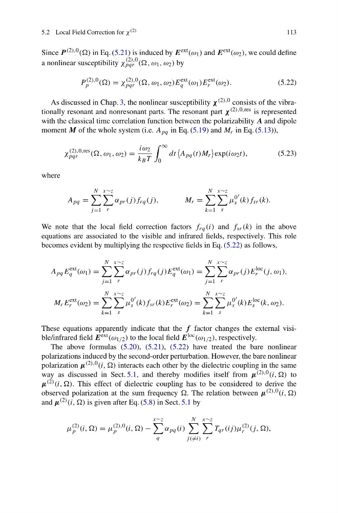
Since P (2),0 (() in Eq. (5.21) is induced by E ext (ω 1 ) and E ext (ω 2 ), we could define
a nonlinear susceptibility χ
(2),0
pqr ((, ω 1 , ω 2 ) by
P
(2),0
p
(() = χ
(2),0
pqr ((, ω 1 , ω 2 )E
ext
q (ω 1 )E
ext
r (ω 2 ).
(5.22)
As discussed in Chap. 3, the nonlinear susceptibility χ (2),0 consists of the vibrationally resonant and nonresonant parts. The resonant part χ (2),0,res is represented
with the classical time correlation function between the polarizability A and dipole
moment M of the whole system (i.e. A pq in Eq. (5.19) and M r in Eq. (5.13)),
χ
(2),0,res
pqr
((, ω 1 , ω 2 ) =
iω 2
k B T
∞
0
dt
A pq (t)M r
exp(iω 2 t),
(5.23)
where
A pq =
N
j =1
x∼z
r
α pr (j )f rq (j ),
M r =
N
k=1
x∼z
s
μ
0
s
(k)f sr (k).
We note that the local field correction factors f rq (i) and f sr (k) in the above
equations are associated to the visible and infrared fields, respectively. This role
becomes evident by multiplying the respective fields in Eq. (5.22) as follows,
A pq E
ext
q (ω 1 ) =
N
j =1
x∼z
r
α pr (j )f rq (j )E
ext
q (ω 1 ) =
N
j =1
x∼z
r
α pr (j )E
loc
r (j, ω 1 ),
M r E
ext
r (ω 2 ) =
N
k=1
x∼z
s
μ
0
s
(k)f sr (k)E
ext
r (ω 2 ) =
N
k=1
x∼z
s
μ
0
s
(k)E
loc
s (k, ω 2 ).
These equations apparently indicate that the f factor changes the external visible/infrared field E ext (ω 1/2 ) to the local field E loc (ω 1/2 ), respectively.
The above formulas (5.20), (5.21), (5.22) have treated the bare nonlinear
polarizations induced by the second-order perturbation. However, the bare nonlinear
polarization μ (2),0 (i, ,) interacts each other by the dielectric coupling in the same
way as discussed in Sect. 5.1, and thereby modifies itself from μ (2),0 (i, ,) to
μ (2) (i, ,). This effect of dielectric coupling has to be considered to derive the
observed polarization at the sum frequency . The relation between μ (2),0 (i, ,)
and μ (2) (i, ,) is given after Eq. (5.8) in Sect. 5.1 by
μ
(2)
p (i, ,) = μ
(2),0
p
(i, ,) −
x∼z
q
α pq (i)
N
j ( =i)
x∼z
r
T qr (ij )μ
(2)
r (j, ,),
113
Since P (2),0 (() in Eq. (5.21) is induced by E ext (ω 1 ) and E ext (ω 2 ), we could define
a nonlinear susceptibility χ
(2),0
pqr ((, ω 1 , ω 2 ) by
P
(2),0
p
(() = χ
(2),0
pqr ((, ω 1 , ω 2 )E
ext
q (ω 1 )E
ext
r (ω 2 ).
(5.22)
As discussed in Chap. 3, the nonlinear susceptibility χ (2),0 consists of the vibrationally resonant and nonresonant parts. The resonant part χ (2),0,res is represented
with the classical time correlation function between the polarizability A and dipole
moment M of the whole system (i.e. A pq in Eq. (5.19) and M r in Eq. (5.13)),
χ
(2),0,res
pqr
((, ω 1 , ω 2 ) =
iω 2
k B T
∞
0
dt
A pq (t)M r
exp(iω 2 t),
(5.23)
where
A pq =
N
j =1
x∼z
r
α pr (j )f rq (j ),
M r =
N
k=1
x∼z
s
μ
0
s
(k)f sr (k).
We note that the local field correction factors f rq (i) and f sr (k) in the above
equations are associated to the visible and infrared fields, respectively. This role
becomes evident by multiplying the respective fields in Eq. (5.22) as follows,
A pq E
ext
q (ω 1 ) =
N
j =1
x∼z
r
α pr (j )f rq (j )E
ext
q (ω 1 ) =
N
j =1
x∼z
r
α pr (j )E
loc
r (j, ω 1 ),
M r E
ext
r (ω 2 ) =
N
k=1
x∼z
s
μ
0
s
(k)f sr (k)E
ext
r (ω 2 ) =
N
k=1
x∼z
s
μ
0
s
(k)E
loc
s (k, ω 2 ).
These equations apparently indicate that the f factor changes the external visible/infrared field E ext (ω 1/2 ) to the local field E loc (ω 1/2 ), respectively.
The above formulas (5.20), (5.21), (5.22) have treated the bare nonlinear
polarizations induced by the second-order perturbation. However, the bare nonlinear
polarization μ (2),0 (i, ,) interacts each other by the dielectric coupling in the same
way as discussed in Sect. 5.1, and thereby modifies itself from μ (2),0 (i, ,) to
μ (2) (i, ,). This effect of dielectric coupling has to be considered to derive the
observed polarization at the sum frequency . The relation between μ (2),0 (i, ,)
and μ (2) (i, ,) is given after Eq. (5.8) in Sect. 5.1 by
μ
(2)
p (i, ,) = μ
(2),0
p
(i, ,) −
x∼z
q
α pq (i)
N
j ( =i)
x∼z
r
T qr (ij )μ
(2)
r (j, ,),