

4.3 Time-Dependent Representation
95
· exp
iE m t
¯
h
m|δα pq |n
exp
−iE n t
¯
h
n|δμ r |m
= −
1
Q
m
n( =m)
exp(−βE m ) − exp(−βE n )
E m − E n
m|δα pq |n
n|δμ r |m
− iω 2
∞
0
dt exp(iω 2 t) ·
1
Q
m
n( =m)
exp(−βE m ) − exp(−βE n )
E m − E n
· exp
iE m t
¯
h
m|δα pq |n
exp
−iE n t
¯
h
n|δμ r |m
= βG(0) + iω 2 β
∞
0
dt G(t) exp(iω 2 t).
(4.27)
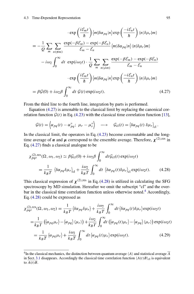
From the third line to the fourth line, integration by parts is performed.
Equation (4.27) is amenable to the classical limit by replacing the canonical correlation function G(t) in Eq. (4.23) with the classical time correlation function [13],
G(t) =
α pq (t) − α
◦
pq ; μ r − μ
◦
r
− −→ G cl (t) =
δα pq (t) δμ r
cl
.
In the classical limit, the operators in Eq. (4.23) become commutable and the longtime average of α and μ correspond to the ensemble average. Therefore, χ (2),res in
Eq. (4.27) finds a classical analogue to be
χ
(2),res
pqr ((, ω 1 , ω 2 ) βG cl (0) + iω 2 β
∞
0
dtG cl (t) exp(iω 2 t)
=
1
k B T
δα pq δμ r
cl
+
iω 2
k B T
∞
0
dt
δα pq (t)δμ r
cl
exp(iω 2 t).
(4.28)
This classical expression of χ (2),res in Eq. (4.28) is utilized in calculating the SFG
spectroscopy by MD simulation. Hereafter we omit the subscript “cl” and the overbar in the classical time correlation function unless otherwise noted. 4 Accordingly,
Eq. (4.28) could be expressed as
χ
(2),res
pqr ((, ω 1 , ω 2 ) =
1
k B T
δα pq δμ r
+
iω 2
k B T
∞
0
dt
δα pq (t)δμ r
exp(iω 2 t)
=
1
k B T
α pq μ r
−
α pq
μ r
+
iω 2
k B T
∞
0
dt
α pq (t)μ r
−
α pq
μ r
exp(iω 2 t)
=
1
k B T
α pq μ r
+
iω 2
k B T
∞
0
dt
α pq (t)μ r
exp(iω 2 t).
(4.29)
4 In the classical mechanics, the distinction between quantum average A and statistical average A
in Sect. 3.1 disappears. Accordingly the classical time correlation function A(t)B cl is equivalent
to A(t)B.
95
· exp
iE m t
¯
h
m|δα pq |n
exp
−iE n t
¯
h
n|δμ r |m
= −
1
Q
m
n( =m)
exp(−βE m ) − exp(−βE n )
E m − E n
m|δα pq |n
n|δμ r |m
− iω 2
∞
0
dt exp(iω 2 t) ·
1
Q
m
n( =m)
exp(−βE m ) − exp(−βE n )
E m − E n
· exp
iE m t
¯
h
m|δα pq |n
exp
−iE n t
¯
h
n|δμ r |m
= βG(0) + iω 2 β
∞
0
dt G(t) exp(iω 2 t).
(4.27)
From the third line to the fourth line, integration by parts is performed.
Equation (4.27) is amenable to the classical limit by replacing the canonical correlation function G(t) in Eq. (4.23) with the classical time correlation function [13],
G(t) =
α pq (t) − α
◦
pq ; μ r − μ
◦
r
− −→ G cl (t) =
δα pq (t) δμ r
cl
.
In the classical limit, the operators in Eq. (4.23) become commutable and the longtime average of α and μ correspond to the ensemble average. Therefore, χ (2),res in
Eq. (4.27) finds a classical analogue to be
χ
(2),res
pqr ((, ω 1 , ω 2 ) βG cl (0) + iω 2 β
∞
0
dtG cl (t) exp(iω 2 t)
=
1
k B T
δα pq δμ r
cl
+
iω 2
k B T
∞
0
dt
δα pq (t)δμ r
cl
exp(iω 2 t).
(4.28)
This classical expression of χ (2),res in Eq. (4.28) is utilized in calculating the SFG
spectroscopy by MD simulation. Hereafter we omit the subscript “cl” and the overbar in the classical time correlation function unless otherwise noted. 4 Accordingly,
Eq. (4.28) could be expressed as
χ
(2),res
pqr ((, ω 1 , ω 2 ) =
1
k B T
δα pq δμ r
+
iω 2
k B T
∞
0
dt
δα pq (t)δμ r
exp(iω 2 t)
=
1
k B T
α pq μ r
−
α pq
μ r
+
iω 2
k B T
∞
0
dt
α pq (t)μ r
−
α pq
μ r
exp(iω 2 t)
=
1
k B T
α pq μ r
+
iω 2
k B T
∞
0
dt
α pq (t)μ r
exp(iω 2 t).
(4.29)
4 In the classical mechanics, the distinction between quantum average A and statistical average A
in Sect. 3.1 disappears. Accordingly the classical time correlation function A(t)B cl is equivalent
to A(t)B.