

4.4.1 Configurational Sampling
MD at fixed temperature, volume, and particle number (NVT) is the most common
way to obtain a canonical ensemble, the structures (configurations) of which can be
used to obtain a statistical average of a property in the thermodynamic equilibrium
at a given temperature. The MD simulation must be sufficiently long to explore the
relevant regions of the configurational space, i.e., provide ergodicity. It is an open
problem to predict a priory when this condition is satisfied. The property, e.g.,
absorption spectrum is then calculated for a set of randomly chosen MD snapshots.
Configurational sampling removes the problem that a single point calculation only
considers the structure of an arbitrary local minimum that may or may not well
represent the average structure at room temperature. Furthermore, it provides an
estimate for the line broadening and the effect of superposition of different
conformations that are occupied in the thermodynamic equilibrium. Examples
can be found for the calculation of solvent shifts of acrolein in water [113–115],
the opsin shift of the absorption maximum of the retinal chromophore in different
rhodopsin proteins [116–118], the calculation of NMR chemical shifts [119], and
the calculation of vertical detachment energies for microsolvated ions [120].
Another powerful application of configurational sampling is to analyze the
correlation between a calculated property and structural parameters. For retinal
chromophore, e.g., a strong correlation can be found between the bond-length
alternation of the chromophore and the absorption maximum [116].
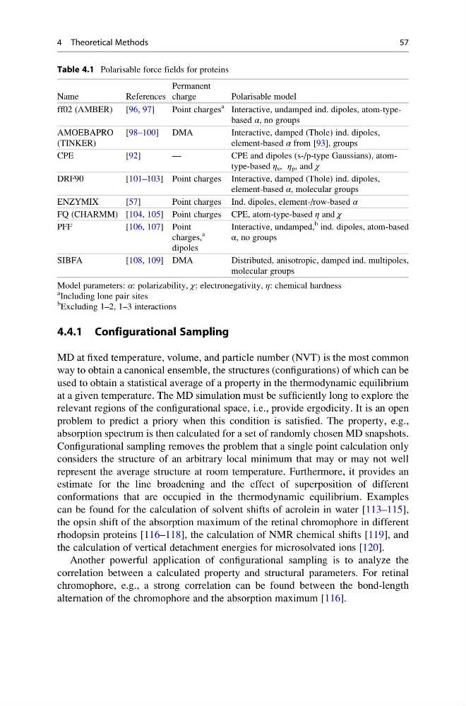
Table 4.1 Polarisable force fields for proteins
Name
References
Permanent
charge
Polarisable model
ff02 (AMBER) [96, 97]
Point charges
a Interactive, undamped ind. dipoles, atom-typebased α, no groups
AMOEBAPRO
(TINKER)
[98–100] DMA
Interactive, damped (Thole) ind. dipoles,
element-based α from [93], groups
CPE
[92]
—
CPE and dipoles (s-/p-type Gaussians), atomtype-based η s , η p , and χ
DRF90
[101–103] Point charges Interactive, damped (Thole) ind. dipoles,
element-based α, molecular groups
ENZYMIX
[57]
Point charges Ind. dipoles, element-/row-based α
FQ (CHARMM) [104, 105] Point charges CPE, atom-type-based η and χ
PFF
[106, 107] Point
charges,
a
dipoles
Interactive, undamped,
b ind. dipoles, atom-based
α, no groups
SIBFA
[108, 109] DMA
Distributed, anisotropic, damped ind. multipoles,
molecular groups
Model parameters: α: polarizability, χ: electronegativity, η: chemical hardness
a
Including lone pair sites
b
Excluding 1–2, 1–3 interactions
4 Theoretical Methods
57
MD at fixed temperature, volume, and particle number (NVT) is the most common
way to obtain a canonical ensemble, the structures (configurations) of which can be
used to obtain a statistical average of a property in the thermodynamic equilibrium
at a given temperature. The MD simulation must be sufficiently long to explore the
relevant regions of the configurational space, i.e., provide ergodicity. It is an open
problem to predict a priory when this condition is satisfied. The property, e.g.,
absorption spectrum is then calculated for a set of randomly chosen MD snapshots.
Configurational sampling removes the problem that a single point calculation only
considers the structure of an arbitrary local minimum that may or may not well
represent the average structure at room temperature. Furthermore, it provides an
estimate for the line broadening and the effect of superposition of different
conformations that are occupied in the thermodynamic equilibrium. Examples
can be found for the calculation of solvent shifts of acrolein in water [113–115],
the opsin shift of the absorption maximum of the retinal chromophore in different
rhodopsin proteins [116–118], the calculation of NMR chemical shifts [119], and
the calculation of vertical detachment energies for microsolvated ions [120].
Another powerful application of configurational sampling is to analyze the
correlation between a calculated property and structural parameters. For retinal
chromophore, e.g., a strong correlation can be found between the bond-length
alternation of the chromophore and the absorption maximum [116].
Table 4.1 Polarisable force fields for proteins
Name
References
Permanent
charge
Polarisable model
ff02 (AMBER) [96, 97]
Point charges
a Interactive, undamped ind. dipoles, atom-typebased α, no groups
AMOEBAPRO
(TINKER)
[98–100] DMA
Interactive, damped (Thole) ind. dipoles,
element-based α from [93], groups
CPE
[92]
—
CPE and dipoles (s-/p-type Gaussians), atomtype-based η s , η p , and χ
DRF90
[101–103] Point charges Interactive, damped (Thole) ind. dipoles,
element-based α, molecular groups
ENZYMIX
[57]
Point charges Ind. dipoles, element-/row-based α
FQ (CHARMM) [104, 105] Point charges CPE, atom-type-based η and χ
PFF
[106, 107] Point
charges,
a
dipoles
Interactive, undamped,
b ind. dipoles, atom-based
α, no groups
SIBFA
[108, 109] DMA
Distributed, anisotropic, damped ind. multipoles,
molecular groups
Model parameters: α: polarizability, χ: electronegativity, η: chemical hardness
a
Including lone pair sites
b
Excluding 1–2, 1–3 interactions
4 Theoretical Methods
57