

full-CI limit. This is a direct consequence of the implicit incorporation of dynamic
electron correlation in the parameterization and the resulting smaller two-electron
integrals [53, 54]. OM2/MRCI hence recovers both dynamic and static correlation
in a balanced way and performs well in the calculation of π À π* excitations with
partial CT character. It has been applied, e.g., to the retinal chromophore and the
related colour tuning of rhodopsins as well as to calculations on the green fluorescent protein (GFP), where it outperforms TDDFT with GGA and conventional
hybrid functionals and correctly describes excitation-induced CT, response to
electrostatic and steric interactions and excited-state geometries [23, 55, 56]. For
nonadiabatic excited-state dynamics simulations, the electronic time-propagation
and the surface-hopping algorithm have been implemented and applied to many
systems (see Sect. 4.4).
4.3
QM/MM and Beyond
To understand the photophysical properties of organic chromophores, it is inevitable to study their intrinsic properties in vacuo. For practical applications, however,
the influence of the environment on these properties is at least as important. This
applies in particular to biological chromophores inside proteins, whose optical
properties are regulated by the specific steric and electrostatic interactions with
the protein. Approaches to account for these and further interactions (static
polarisation, dispersion, charge exchange) will be discussed in this section. The
main idea is to combine different levels of theory for the optically active part of the
system and the environment. The most prominent scheme employs a QM method
for the description of the active part and a classical molecular dynamics (MM) force
field for the description of the environment (QM/MM) [57]. The MM force field
can be extended to describe polarisation effects and coupled to a continuumelectrostatic model to describe the long-range effect of bulk solvation.
4.3.1 Schemes
Traditionally, additive (QM/MM [57]) and subtractive (ONIOM [58]) schemes are
distinguished. The latter is conceptually clear and applicable in a general context. It
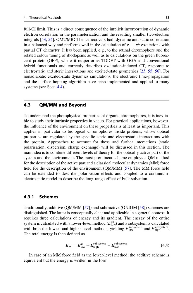
requires three calculations of energy and its gradient. The energy of the entire
system is calculated with a lower-level method (E low
all ) and a subsystem is calculated
with both the lower- and higher-level methods, yielding E low
subsystem and E high
subsystem .
The total energy is then defined as
E tot ¼ E
all
low þ E
subsystem
high
À E
subsystem
low
(4.4)
In case of an MM force field as the lower-level method, the additive scheme is
equivalent but the energy is written in the form
4 Theoretical Methods
53
electron correlation in the parameterization and the resulting smaller two-electron
integrals [53, 54]. OM2/MRCI hence recovers both dynamic and static correlation
in a balanced way and performs well in the calculation of π À π* excitations with
partial CT character. It has been applied, e.g., to the retinal chromophore and the
related colour tuning of rhodopsins as well as to calculations on the green fluorescent protein (GFP), where it outperforms TDDFT with GGA and conventional
hybrid functionals and correctly describes excitation-induced CT, response to
electrostatic and steric interactions and excited-state geometries [23, 55, 56]. For
nonadiabatic excited-state dynamics simulations, the electronic time-propagation
and the surface-hopping algorithm have been implemented and applied to many
systems (see Sect. 4.4).
4.3
QM/MM and Beyond
To understand the photophysical properties of organic chromophores, it is inevitable to study their intrinsic properties in vacuo. For practical applications, however,
the influence of the environment on these properties is at least as important. This
applies in particular to biological chromophores inside proteins, whose optical
properties are regulated by the specific steric and electrostatic interactions with
the protein. Approaches to account for these and further interactions (static
polarisation, dispersion, charge exchange) will be discussed in this section. The
main idea is to combine different levels of theory for the optically active part of the
system and the environment. The most prominent scheme employs a QM method
for the description of the active part and a classical molecular dynamics (MM) force
field for the description of the environment (QM/MM) [57]. The MM force field
can be extended to describe polarisation effects and coupled to a continuumelectrostatic model to describe the long-range effect of bulk solvation.
4.3.1 Schemes
Traditionally, additive (QM/MM [57]) and subtractive (ONIOM [58]) schemes are
distinguished. The latter is conceptually clear and applicable in a general context. It
requires three calculations of energy and its gradient. The energy of the entire
system is calculated with a lower-level method (E low
all ) and a subsystem is calculated
with both the lower- and higher-level methods, yielding E low
subsystem and E high
subsystem .
The total energy is then defined as
E tot ¼ E
all
low þ E
subsystem
high
À E
subsystem
low
(4.4)
In case of an MM force field as the lower-level method, the additive scheme is
equivalent but the energy is written in the form
4 Theoretical Methods
53