

548
V. N. Pustovit and T. V. Shahbazyan
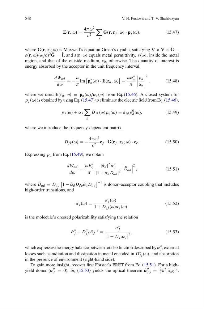
E(r, ω) =
4πω 2
c 2
j
G(r, r j ; ω) · p j (ω),
(15.47)
where G(r, r √ ; ω) is Maxwell’s equation Green’s dyadic, satisfying ∇ × ∇ × ˆ
G −
ε(r, ω)(ω/c) 2 ˆ
G = ˆ
I, and ε(r, ω) equals metal permittivity, ε(ω), inside the metal
region, and that of the outside medium, ε 0 , otherwise. The quantity of interest is
energy absorbed by the acceptor in the unit frequency interval,
dW ad
dω
= −
ω
π
Im
p
∗
a (ω) · E(r a , ω)
=
ωα √√
a
π
p a
α a
2
,
(15.48)
where we used E(r a , ω) = p a (ω)/α a (ω) from Eq. (15.46). A closed system for
p j (ω) is obtained by using Eq. (15.47) to eliminate the electric field from Eq. (15.46),
p j (ω) + α j
k
D jk (ω) p k (ω) = δ jd p
0
d (ω),
(15.49)
where we introduce the frequency-dependent matrix
D jk (ω) = −
4πω 2
c 2 e j · G(r j , r k ; ω) · e k .
(15.50)
Expressing p a from Eq. (15.49), we obtain
dW ad
dω
=
ωE 2
0
π
| ˜
α d |
2
α √√
a
|1 + α a D aa | 2
˜
D ad
2 ,
(15.51)
where ˜
D ad = D ad
1 − ˜
α d D da ˜
α a D ad
−1 is donor–acceptor coupling that includes
high-order transitions, and
˜
α j (ω) =
α j (ω)
1 + D j j (ω)α j (ω)
(15.52)
is the molecule’s dressed polarizability satisfying the relation
˜
α
√√
j + D
√√
j j | ˜
α j |
2
=
α √√
j
1 + D j j α j
2 ,
(15.53)
which expresses the energy balance between total extinction described by ˜
α √√
j , external
losses such as radiation and dissipation in metal encoded in D √√
j j (ω), and absorption
in the presence of environment (right-hand side).
To gain more insight, recover first Förster’s FRET from Eq. (15.51). For a highyield donor (α √√
d = 0), Eq. (15.53) yields the optical theorem ˜
α √√
d0 =
2
3 k 3 | ˜
α d0 | 2 ,
V. N. Pustovit and T. V. Shahbazyan
E(r, ω) =
4πω 2
c 2
j
G(r, r j ; ω) · p j (ω),
(15.47)
where G(r, r √ ; ω) is Maxwell’s equation Green’s dyadic, satisfying ∇ × ∇ × ˆ
G −
ε(r, ω)(ω/c) 2 ˆ
G = ˆ
I, and ε(r, ω) equals metal permittivity, ε(ω), inside the metal
region, and that of the outside medium, ε 0 , otherwise. The quantity of interest is
energy absorbed by the acceptor in the unit frequency interval,
dW ad
dω
= −
ω
π
Im
p
∗
a (ω) · E(r a , ω)
=
ωα √√
a
π
p a
α a
2
,
(15.48)
where we used E(r a , ω) = p a (ω)/α a (ω) from Eq. (15.46). A closed system for
p j (ω) is obtained by using Eq. (15.47) to eliminate the electric field from Eq. (15.46),
p j (ω) + α j
k
D jk (ω) p k (ω) = δ jd p
0
d (ω),
(15.49)
where we introduce the frequency-dependent matrix
D jk (ω) = −
4πω 2
c 2 e j · G(r j , r k ; ω) · e k .
(15.50)
Expressing p a from Eq. (15.49), we obtain
dW ad
dω
=
ωE 2
0
π
| ˜
α d |
2
α √√
a
|1 + α a D aa | 2
˜
D ad
2 ,
(15.51)
where ˜
D ad = D ad
1 − ˜
α d D da ˜
α a D ad
−1 is donor–acceptor coupling that includes
high-order transitions, and
˜
α j (ω) =
α j (ω)
1 + D j j (ω)α j (ω)
(15.52)
is the molecule’s dressed polarizability satisfying the relation
˜
α
√√
j + D
√√
j j | ˜
α j |
2
=
α √√
j
1 + D j j α j
2 ,
(15.53)
which expresses the energy balance between total extinction described by ˜
α √√
j , external
losses such as radiation and dissipation in metal encoded in D √√
j j (ω), and absorption
in the presence of environment (right-hand side).
To gain more insight, recover first Förster’s FRET from Eq. (15.51). For a highyield donor (α √√
d = 0), Eq. (15.53) yields the optical theorem ˜
α √√
d0 =
2
3 k 3 | ˜
α d0 | 2 ,