

404
B. Igne and E. W. Ciurczak
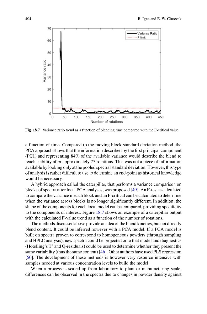
Fig. 18.7 Variance ratio trend as a function of blending time compared with the F-critical value
a function of time. Compared to the moving block standard deviation method, the
PCA approach shows that the information described by the first principal component
(PC1) and representing 84% of the available variance would describe the blend to
reach stability after approximately 75 rotations. This was not a piece of information
available by looking only at the pooled spectral standard deviation. However, this type
of analysis is rather difficult to use to determine an end-point as historical knowledge
would be necessary.
A hybrid approach called the caterpillar, that performs a variance comparison on
blocks of spectra after local PCA analyses, was proposed [49]. An F-test is calculated
to compare the variance in each block and an F-critical can be calculated to determine
when the variance across blocks is no longer significantly different. In addition, the
shape of the components for each local model can be compared, providing specificity
to the components of interest. Figure 18.7 shows an example of a caterpillar output
with the calculated F-value trend as a function of the number of rotations.
The methods discussed above provide an idea of the blend kinetics, but not directly
blend content. It could be inferred however with a PCA model. If a PCA model is
built on spectra proven to correspond to homogeneous powders (through sampling
and HPLC analysis), new spectra could be projected onto that model and diagnostics
(Hotelling’s T
2 and Q-residuals) could be used to determine whether they present the
same variability (thus the same content) [46]. Other authors have used PLS regression
[50]. The development of these methods is however very resource intensive with
samples needed at various concentration levels to build the model.
When a process is scaled up from laboratory to plant or manufacturing scale,
differences can be observed in the spectra due to changes in powder density against
B. Igne and E. W. Ciurczak
Fig. 18.7 Variance ratio trend as a function of blending time compared with the F-critical value
a function of time. Compared to the moving block standard deviation method, the
PCA approach shows that the information described by the first principal component
(PC1) and representing 84% of the available variance would describe the blend to
reach stability after approximately 75 rotations. This was not a piece of information
available by looking only at the pooled spectral standard deviation. However, this type
of analysis is rather difficult to use to determine an end-point as historical knowledge
would be necessary.
A hybrid approach called the caterpillar, that performs a variance comparison on
blocks of spectra after local PCA analyses, was proposed [49]. An F-test is calculated
to compare the variance in each block and an F-critical can be calculated to determine
when the variance across blocks is no longer significantly different. In addition, the
shape of the components for each local model can be compared, providing specificity
to the components of interest. Figure 18.7 shows an example of a caterpillar output
with the calculated F-value trend as a function of the number of rotations.
The methods discussed above provide an idea of the blend kinetics, but not directly
blend content. It could be inferred however with a PCA model. If a PCA model is
built on spectra proven to correspond to homogeneous powders (through sampling
and HPLC analysis), new spectra could be projected onto that model and diagnostics
(Hotelling’s T
2 and Q-residuals) could be used to determine whether they present the
same variability (thus the same content) [46]. Other authors have used PLS regression
[50]. The development of these methods is however very resource intensive with
samples needed at various concentration levels to build the model.
When a process is scaled up from laboratory to plant or manufacturing scale,
differences can be observed in the spectra due to changes in powder density against