

184
K. M. Sørensen et al.
0
100
200
300
Linear index
-0.2
0
0.2
Variety scores PC1
0
100
200
300
Linear index
-2
0
2
Positon scores PC1
850
900 950 1000 1050
Wavelength [nm]
-0.2
0
0.2
0.4
Variety loadings PC1
850
900 950 1000 1050
Wavelength [nm]
-0.4
-0.2
0
0.2
0.4
Positon loadings PC1
a
b
c
d
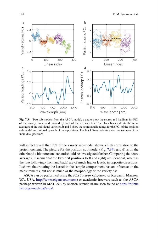
Fig. 7.34 Two sub-models from the ASCA model. a and c show the scores and loadings for PC1
of the variety model and colored by each of the five varieties. The black lines indicate the score
averages of the individual varieties. b and d show the scores and loadings for the PC1 of the position
sub-model and colored by each of the 4 positions. The black lines indicate the score averages of the
individual positions
will in fact reveal that PC1 of the variety sub-model shows a high correlation to the
protein content. The picture for the position sub-model (Fig. 7.34b and d) is on the
other hand a bit more unclear and should be investigated further. Comparing the score
averages, it seems that the two first positions (left and right) are identical, whereas
the two following (front and back) are of much higher levels, in opposite directions.
It shows that rotating the kernel in the sample compartment has an influence on the
measurements, but not as much as the morphology of the variety has.
ASCA can be performed using the PLS Toolbox (Eigenvector Research, Manson,
WA, USA, http://www.eigenvector.com) or academic freeware such as the ASCA
package written in MATLAB by Morten Arendt Rasmussen found at https://bitbuc
ket.org/modelscat/asca/.
K. M. Sørensen et al.
0
100
200
300
Linear index
-0.2
0
0.2
Variety scores PC1
0
100
200
300
Linear index
-2
0
2
Positon scores PC1
850
900 950 1000 1050
Wavelength [nm]
-0.2
0
0.2
0.4
Variety loadings PC1
850
900 950 1000 1050
Wavelength [nm]
-0.4
-0.2
0
0.2
0.4
Positon loadings PC1
a
b
c
d
Fig. 7.34 Two sub-models from the ASCA model. a and c show the scores and loadings for PC1
of the variety model and colored by each of the five varieties. The black lines indicate the score
averages of the individual varieties. b and d show the scores and loadings for the PC1 of the position
sub-model and colored by each of the 4 positions. The black lines indicate the score averages of the
individual positions
will in fact reveal that PC1 of the variety sub-model shows a high correlation to the
protein content. The picture for the position sub-model (Fig. 7.34b and d) is on the
other hand a bit more unclear and should be investigated further. Comparing the score
averages, it seems that the two first positions (left and right) are identical, whereas
the two following (front and back) are of much higher levels, in opposite directions.
It shows that rotating the kernel in the sample compartment has an influence on the
measurements, but not as much as the morphology of the variety has.
ASCA can be performed using the PLS Toolbox (Eigenvector Research, Manson,
WA, USA, http://www.eigenvector.com) or academic freeware such as the ASCA
package written in MATLAB by Morten Arendt Rasmussen found at https://bitbuc
ket.org/modelscat/asca/.