

7 NIR Data Exploration and Regression by Chemometrics—A Primer
179
1100
1300
1500
1700
1900
2100
2300
2500
Wavelength [nm]
0
1
2
3
4
5
6
7
8
RMSECV
0
0.1
0.2
0.3
0.4
0.5
0.6
0.7
0.8
0.9
Mean spectra, log(T)
2
3
3
3
6
4
7
3
6
1
3
4
2
2
3
2
3
3
2
Best interval
RMSECV=2.087
2 components
Global model
RMSECV=2.151
3 Components
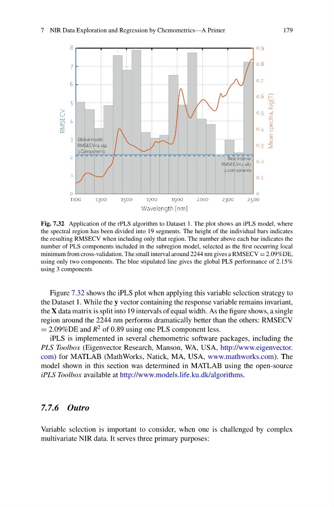
Fig. 7.32 Application of the rPLS algorithm to Dataset 1. The plot shows an iPLS model, where
the spectral region has been divided into 19 segments. The height of the individual bars indicates
the resulting RMSECV when including only that region. The number above each bar indicates the
number of PLS components included in the subregion model, selected as the first occurring local
minimum from cross-validation. The small interval around 2244 nm gives a RMSECV = 2.09%DE,
using only two components. The blue stipulated line gives the global PLS performance of 2.15%
using 3 components
Figure 7.32 shows the iPLS plot when applying this variable selection strategy to
the Dataset 1. While the y vector containing the response variable remains invariant,
the X data matrix is split into 19 intervals of equal width. As the figure shows, a single
region around the 2244 nm performs dramatically better than the others: RMSECV
= 2.09%DE and R
2 of 0.89 using one PLS component less.
iPLS is implemented in several chemometric software packages, including the
PLS Toolbox (Eigenvector Research, Manson, WA, USA, http://www.eigenvector.
com) for MATLAB (MathWorks, Natick, MA, USA, www.mathworks.com). The
model shown in this section was determined in MATLAB using the open-source
iPLS Toolbox available at http://www.models.life.ku.dk/algorithms.
7.7.6 Outro
Variable selection is important to consider, when one is challenged by complex
multivariate NIR data. It serves three primary purposes:
179
1100
1300
1500
1700
1900
2100
2300
2500
Wavelength [nm]
0
1
2
3
4
5
6
7
8
RMSECV
0
0.1
0.2
0.3
0.4
0.5
0.6
0.7
0.8
0.9
Mean spectra, log(T)
2
3
3
3
6
4
7
3
6
1
3
4
2
2
3
2
3
3
2
Best interval
RMSECV=2.087
2 components
Global model
RMSECV=2.151
3 Components
Fig. 7.32 Application of the rPLS algorithm to Dataset 1. The plot shows an iPLS model, where
the spectral region has been divided into 19 segments. The height of the individual bars indicates
the resulting RMSECV when including only that region. The number above each bar indicates the
number of PLS components included in the subregion model, selected as the first occurring local
minimum from cross-validation. The small interval around 2244 nm gives a RMSECV = 2.09%DE,
using only two components. The blue stipulated line gives the global PLS performance of 2.15%
using 3 components
Figure 7.32 shows the iPLS plot when applying this variable selection strategy to
the Dataset 1. While the y vector containing the response variable remains invariant,
the X data matrix is split into 19 intervals of equal width. As the figure shows, a single
region around the 2244 nm performs dramatically better than the others: RMSECV
= 2.09%DE and R
2 of 0.89 using one PLS component less.
iPLS is implemented in several chemometric software packages, including the
PLS Toolbox (Eigenvector Research, Manson, WA, USA, http://www.eigenvector.
com) for MATLAB (MathWorks, Natick, MA, USA, www.mathworks.com). The
model shown in this section was determined in MATLAB using the open-source
iPLS Toolbox available at http://www.models.life.ku.dk/algorithms.
7.7.6 Outro
Variable selection is important to consider, when one is challenged by complex
multivariate NIR data. It serves three primary purposes: