

178
K. M. Sørensen et al.
1100 1300 1500 1700 1900 2100 2300 2500
1
2
3
4
5
6
7
8
9
10
11
12
13
1.00
0.93
0.86
0.79
0.72
0.65
0.58
0.51
0.43
0.36
0.29
0.22
0.15
0.08
0.01
2.582
2.582
2.581
2.476
2.016
1.835
1.767
1.773
1.776
1.780
1.777
1.777
1.777
Wavelength [nm]
Iteration
Regression weight scale
RMSECV per iteration
13 selected variables
3 final variables
2244 nm
1460 nm
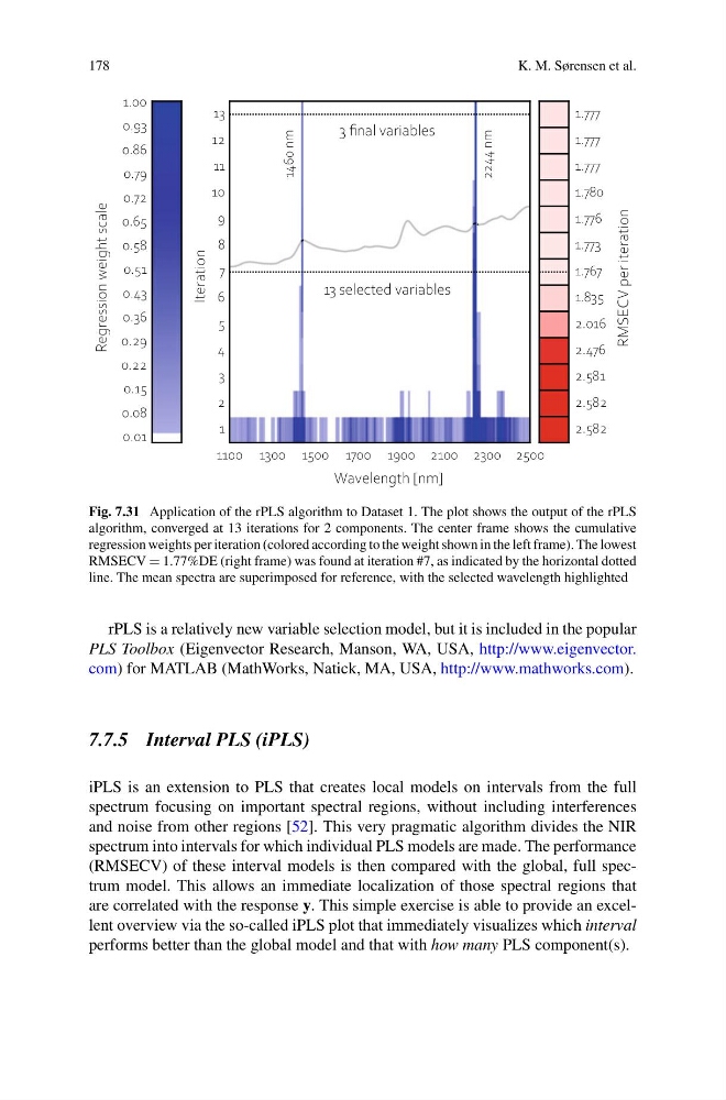
Fig. 7.31 Application of the rPLS algorithm to Dataset 1. The plot shows the output of the rPLS
algorithm, converged at 13 iterations for 2 components. The center frame shows the cumulative
regression weights per iteration (colored according to the weight shown in the left frame). The lowest
RMSECV = 1.77%DE (right frame) was found at iteration #7, as indicated by the horizontal dotted
line. The mean spectra are superimposed for reference, with the selected wavelength highlighted
rPLS is a relatively new variable selection model, but it is included in the popular
PLS Toolbox (Eigenvector Research, Manson, WA, USA, http://www.eigenvector.
com) for MATLAB (MathWorks, Natick, MA, USA, http://www.mathworks.com).
7.7.5 Interval PLS (iPLS)
iPLS is an extension to PLS that creates local models on intervals from the full
spectrum focusing on important spectral regions, without including interferences
and noise from other regions [52]. This very pragmatic algorithm divides the NIR
spectrum into intervals for which individual PLS models are made. The performance
(RMSECV) of these interval models is then compared with the global, full spectrum model. This allows an immediate localization of those spectral regions that
are correlated with the response y. This simple exercise is able to provide an excellent overview via the so-called iPLS plot that immediately visualizes which interval
performs better than the global model and that with how many PLS component(s).
K. M. Sørensen et al.
1100 1300 1500 1700 1900 2100 2300 2500
1
2
3
4
5
6
7
8
9
10
11
12
13
1.00
0.93
0.86
0.79
0.72
0.65
0.58
0.51
0.43
0.36
0.29
0.22
0.15
0.08
0.01
2.582
2.582
2.581
2.476
2.016
1.835
1.767
1.773
1.776
1.780
1.777
1.777
1.777
Wavelength [nm]
Iteration
Regression weight scale
RMSECV per iteration
13 selected variables
3 final variables
2244 nm
1460 nm
Fig. 7.31 Application of the rPLS algorithm to Dataset 1. The plot shows the output of the rPLS
algorithm, converged at 13 iterations for 2 components. The center frame shows the cumulative
regression weights per iteration (colored according to the weight shown in the left frame). The lowest
RMSECV = 1.77%DE (right frame) was found at iteration #7, as indicated by the horizontal dotted
line. The mean spectra are superimposed for reference, with the selected wavelength highlighted
rPLS is a relatively new variable selection model, but it is included in the popular
PLS Toolbox (Eigenvector Research, Manson, WA, USA, http://www.eigenvector.
com) for MATLAB (MathWorks, Natick, MA, USA, http://www.mathworks.com).
7.7.5 Interval PLS (iPLS)
iPLS is an extension to PLS that creates local models on intervals from the full
spectrum focusing on important spectral regions, without including interferences
and noise from other regions [52]. This very pragmatic algorithm divides the NIR
spectrum into intervals for which individual PLS models are made. The performance
(RMSECV) of these interval models is then compared with the global, full spectrum model. This allows an immediate localization of those spectral regions that
are correlated with the response y. This simple exercise is able to provide an excellent overview via the so-called iPLS plot that immediately visualizes which interval
performs better than the global model and that with how many PLS component(s).