

168
K. M. Sørensen et al.
1 2
4
6
8
10
Components in model
40
60
80
100
Cummulative exp. variance [%]
X
y
0
2 0
4 0
6 0
8 0
Glucose measured [%]
0
20
40
60
80
Glcose predicted [%] (2 comps)
1100
1500
2000
2500
Wavelength [nm]
-20
-10
0
10
20
30
Regression
vector
1460 nm
2244 nm
a
b
c
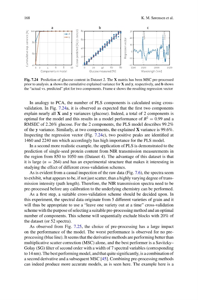
Fig. 7.24 Prediction of glucose content in Dataset 2. The X matrix has been MSC pre-processed
prior to analysis. a shows the cumulative explained variance for X and y, respectively, and b shows
the “actual vs. predicted” plot for two components. Frame c shows the resulting regression vector
In analogy to PCA, the number of PLS components is calculated using crossvalidation. In Fig. 7.24a, it is observed as expected that the first two components
explain nearly all X and y variances (glucose). Indeed, a total of 2 components is
optimal for the model and this results in a model performance of R
2
= 0.99 and a
RMSEC of 2.26% glucose. For the 2 components, the PLS model describes 99.2%
of the y variance. Similarly, at two components, the explained X variance is 99.6%.
Inspecting the regression vector (Fig. 7.24c), two positive peaks are identified at
1460 and 2240 nm which accordingly has high importance for the PLS model.
In a second more realistic example, the application of PLS is demonstrated to the
prediction of single-seed protein content from NIR transmission measurements in
the region from 850 to 1050 nm (Dataset 4). The advantage of this dataset is that
it is large (n = 264) and has an experimental structure that makes it interesting in
studying the effect of different cross-validation schemes.
As is evident from a casual inspection of the raw data (Fig. 7.6), the spectra seem
to exhibit, what appears to be, if not just scatter, than a highly varying degree of transmission intensity (path length). Therefore, the NIR transmission spectra need to be
pre-processed before any calibration to the underlying chemistry can be performed.
As a first step, a suitable cross-validation scheme should be decided upon. In
this experiment, the spectral data originate from 5 different varieties of grain and it
will thus be appropriate to use a “leave one variety out at a time” cross-validation
scheme with the purpose of selecting a suitable pre-processing method and an optimal
number of components. This scheme will sequentially exclude blocks with 20% of
the dataset (or 52 spectra).
As observed from Fig. 7.25, the choice of pre-processing has a large impact
on the performance of the model. The worst performance is observed for no preprocessing (blue line). It seems that the derivative methods are performing better than
multiplicative scatter correction (MSC) alone, and the best performer is a Savitzky–
Golay (SG) filter of second order with a width of 7 spectral variables (corresponding
to 14 nm). The best performing model, and that quite significantly, is a combination of
a second derivative and a subsequent MSC [45]. Combining pre-processing methods
can indeed produce more accurate models, as is seen here. The example here is a
K. M. Sørensen et al.
1 2
4
6
8
10
Components in model
40
60
80
100
Cummulative exp. variance [%]
X
y
0
2 0
4 0
6 0
8 0
Glucose measured [%]
0
20
40
60
80
Glcose predicted [%] (2 comps)
1100
1500
2000
2500
Wavelength [nm]
-20
-10
0
10
20
30
Regression
vector
1460 nm
2244 nm
a
b
c
Fig. 7.24 Prediction of glucose content in Dataset 2. The X matrix has been MSC pre-processed
prior to analysis. a shows the cumulative explained variance for X and y, respectively, and b shows
the “actual vs. predicted” plot for two components. Frame c shows the resulting regression vector
In analogy to PCA, the number of PLS components is calculated using crossvalidation. In Fig. 7.24a, it is observed as expected that the first two components
explain nearly all X and y variances (glucose). Indeed, a total of 2 components is
optimal for the model and this results in a model performance of R
2
= 0.99 and a
RMSEC of 2.26% glucose. For the 2 components, the PLS model describes 99.2%
of the y variance. Similarly, at two components, the explained X variance is 99.6%.
Inspecting the regression vector (Fig. 7.24c), two positive peaks are identified at
1460 and 2240 nm which accordingly has high importance for the PLS model.
In a second more realistic example, the application of PLS is demonstrated to the
prediction of single-seed protein content from NIR transmission measurements in
the region from 850 to 1050 nm (Dataset 4). The advantage of this dataset is that
it is large (n = 264) and has an experimental structure that makes it interesting in
studying the effect of different cross-validation schemes.
As is evident from a casual inspection of the raw data (Fig. 7.6), the spectra seem
to exhibit, what appears to be, if not just scatter, than a highly varying degree of transmission intensity (path length). Therefore, the NIR transmission spectra need to be
pre-processed before any calibration to the underlying chemistry can be performed.
As a first step, a suitable cross-validation scheme should be decided upon. In
this experiment, the spectral data originate from 5 different varieties of grain and it
will thus be appropriate to use a “leave one variety out at a time” cross-validation
scheme with the purpose of selecting a suitable pre-processing method and an optimal
number of components. This scheme will sequentially exclude blocks with 20% of
the dataset (or 52 spectra).
As observed from Fig. 7.25, the choice of pre-processing has a large impact
on the performance of the model. The worst performance is observed for no preprocessing (blue line). It seems that the derivative methods are performing better than
multiplicative scatter correction (MSC) alone, and the best performer is a Savitzky–
Golay (SG) filter of second order with a width of 7 spectral variables (corresponding
to 14 nm). The best performing model, and that quite significantly, is a combination of
a second derivative and a subsequent MSC [45]. Combining pre-processing methods
can indeed produce more accurate models, as is seen here. The example here is a