

7 NIR Data Exploration and Regression by Chemometrics—A Primer
159
included in each step of the algorithm to find the relevant T from X. This is equivalent to going into the supermarket with the menu in hand and therefore having the
opportunity to buy exactly the items you need. Thus, it is not necessary to ensure
that all systematic information in X is represented in T, but it is enough to extract
the information relevant to (or correlating with) y. This principle, which makes the
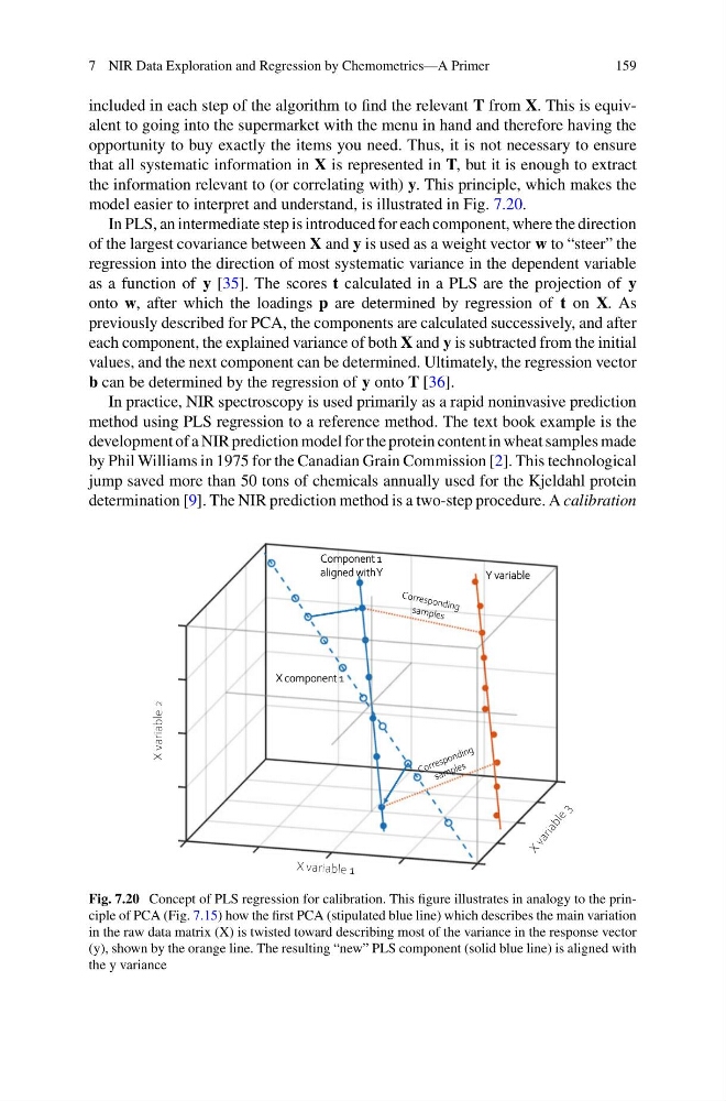
model easier to interpret and understand, is illustrated in Fig. 7.20.
In PLS, an intermediate step is introduced for each component, where the direction
of the largest covariance between X and y is used as a weight vector w to “steer” the
regression into the direction of most systematic variance in the dependent variable
as a function of y [35]. The scores t calculated in a PLS are the projection of y
onto w, after which the loadings p are determined by regression of t on X. As
previously described for PCA, the components are calculated successively, and after
each component, the explained variance of both X and y is subtracted from the initial
values, and the next component can be determined. Ultimately, the regression vector
b can be determined by the regression of y onto T [36].
In practice, NIR spectroscopy is used primarily as a rapid noninvasive prediction
method using PLS regression to a reference method. The text book example is the
development of a NIR prediction model for the protein content in wheat samples made
by Phil Williams in 1975 for the Canadian Grain Commission [2]. This technological
jump saved more than 50 tons of chemicals annually used for the Kjeldahl protein
determination [9]. The NIR prediction method is a two-step procedure. A calibration
X variable 2
Y variable
X component 1
Component 1
aligned withY
Fig. 7.20 Concept of PLS regression for calibration. This figure illustrates in analogy to the principle of PCA (Fig. 7.15) how the first PCA (stipulated blue line) which describes the main variation
in the raw data matrix (X) is twisted toward describing most of the variance in the response vector
(y), shown by the orange line. The resulting “new” PLS component (solid blue line) is aligned with
the y variance
159
included in each step of the algorithm to find the relevant T from X. This is equivalent to going into the supermarket with the menu in hand and therefore having the
opportunity to buy exactly the items you need. Thus, it is not necessary to ensure
that all systematic information in X is represented in T, but it is enough to extract
the information relevant to (or correlating with) y. This principle, which makes the
model easier to interpret and understand, is illustrated in Fig. 7.20.
In PLS, an intermediate step is introduced for each component, where the direction
of the largest covariance between X and y is used as a weight vector w to “steer” the
regression into the direction of most systematic variance in the dependent variable
as a function of y [35]. The scores t calculated in a PLS are the projection of y
onto w, after which the loadings p are determined by regression of t on X. As
previously described for PCA, the components are calculated successively, and after
each component, the explained variance of both X and y is subtracted from the initial
values, and the next component can be determined. Ultimately, the regression vector
b can be determined by the regression of y onto T [36].
In practice, NIR spectroscopy is used primarily as a rapid noninvasive prediction
method using PLS regression to a reference method. The text book example is the
development of a NIR prediction model for the protein content in wheat samples made
by Phil Williams in 1975 for the Canadian Grain Commission [2]. This technological
jump saved more than 50 tons of chemicals annually used for the Kjeldahl protein
determination [9]. The NIR prediction method is a two-step procedure. A calibration
X variable 2
Y variable
X component 1
Component 1
aligned withY
Fig. 7.20 Concept of PLS regression for calibration. This figure illustrates in analogy to the principle of PCA (Fig. 7.15) how the first PCA (stipulated blue line) which describes the main variation
in the raw data matrix (X) is twisted toward describing most of the variance in the response vector
(y), shown by the orange line. The resulting “new” PLS component (solid blue line) is aligned with
the y variance