

158
K. M. Sørensen et al.
X
E
=
+
n
m
f
f
n
m
n
m
T·P
T
n
1
=
n
f 1
+
n
1
T·b
T
y
q
f
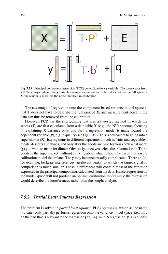
Fig. 7.19 Principal component regression (PCR) generalized to a y variable. The score space from
a PCA is projected onto the y variables using a regression vector b. b does not use the full space of
X; the residuals E will be the noise, not used in calibration
The advantage of regression onto the component-based variance model space is
that T does not have to describe the full rank of X, and measurement noise in the
data can thus be removed from the calibration.
However, PCR has the shortcoming that it is a two-step method in which the
scores (T) are first calculated from a data table X (e.g., the NIR spectra), focusing
on explaining X variance only, and then a regression model is made toward the
dependent variable (y), e.g., a quality (see Fig. 7.19). This is equivalent to going into a
supermarket (X), buying items in different departments such as fruits and vegetables,
meats, desserts and wines, and only after the goods are paid for you know what menu
(y) you want to make for dinner. Obviously, once you select the information in T (the
goods in the supermarket) without thinking about what it should be used for, then the
calibration model that relates T to y may be unnecessarily complicated. There could,
for example, be large interferences (irrelevant peaks) to which the target signal in
comparison is much smaller. These interferences will contain most of the variation
expressed in the principal components calculated from the data. Hence, regression on
the model space will not produce an optimal calibration model since the regression
would describe the interferences rather than the sought analyte.
7.5.2 Partial Least Squares Regression
The problem is solved in partial least squares (PLS) regression, which as the name
indicates only partially performs regression onto the variance model space, i.e., only
on the part that is relevant to the regression [32, 34]. In PLS regression, y is explicitly
K. M. Sørensen et al.
X
E
=
+
n
m
f
f
n
m
n
m
T·P
T
n
1
=
n
f 1
+
n
1
T·b
T
y
q
f
Fig. 7.19 Principal component regression (PCR) generalized to a y variable. The score space from
a PCA is projected onto the y variables using a regression vector b. b does not use the full space of
X; the residuals E will be the noise, not used in calibration
The advantage of regression onto the component-based variance model space is
that T does not have to describe the full rank of X, and measurement noise in the
data can thus be removed from the calibration.
However, PCR has the shortcoming that it is a two-step method in which the
scores (T) are first calculated from a data table X (e.g., the NIR spectra), focusing
on explaining X variance only, and then a regression model is made toward the
dependent variable (y), e.g., a quality (see Fig. 7.19). This is equivalent to going into a
supermarket (X), buying items in different departments such as fruits and vegetables,
meats, desserts and wines, and only after the goods are paid for you know what menu
(y) you want to make for dinner. Obviously, once you select the information in T (the
goods in the supermarket) without thinking about what it should be used for, then the
calibration model that relates T to y may be unnecessarily complicated. There could,
for example, be large interferences (irrelevant peaks) to which the target signal in
comparison is much smaller. These interferences will contain most of the variation
expressed in the principal components calculated from the data. Hence, regression on
the model space will not produce an optimal calibration model since the regression
would describe the interferences rather than the sought analyte.
7.5.2 Partial Least Squares Regression
The problem is solved in partial least squares (PLS) regression, which as the name
indicates only partially performs regression onto the variance model space, i.e., only
on the part that is relevant to the regression [32, 34]. In PLS regression, y is explicitly