

152
K. M. Sørensen et al.
-1
-0.5
0
0.5
1
Scores, component 1 (88.0% var. exp.)
-0.4
-0.3
-0.2
-0.1
0
0.1
0.2
0.3
0.4
Scores, component 2 (11.6% var. exp.)
1100 1300 1500 1700 1900 2100 2300 2500
Wavelength [nm]
-0.05
0
0.05
0.1
0.15
PCA Loadings
PC 1
PC 2
#43
#107
#224
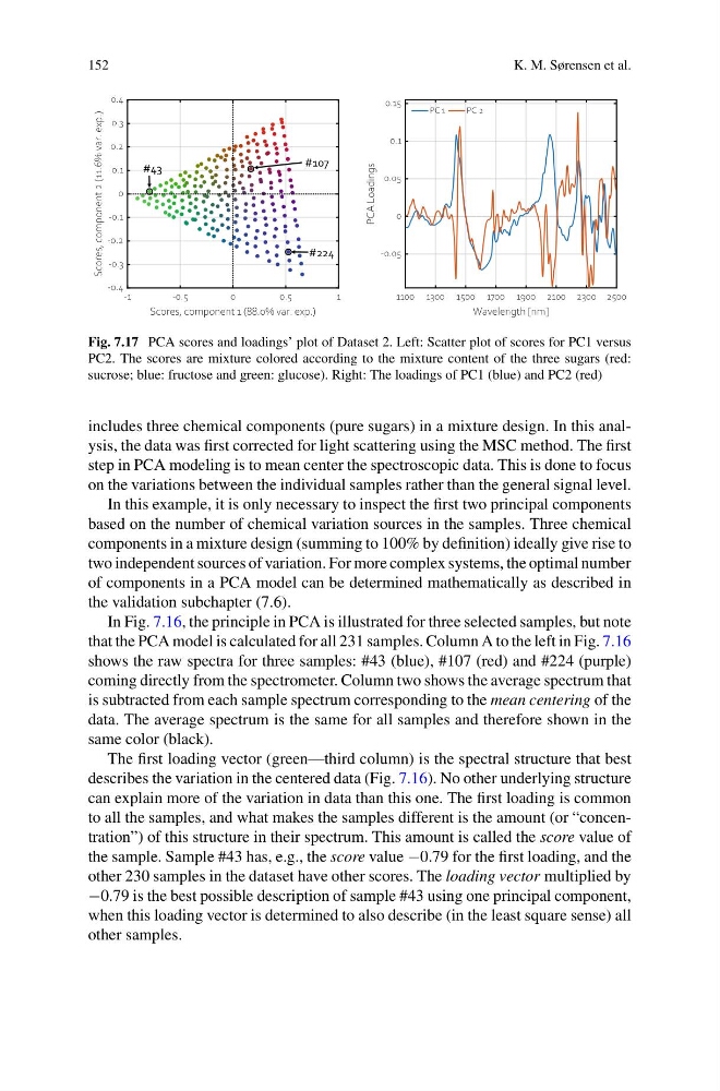
Fig. 7.17 PCA scores and loadings’ plot of Dataset 2. Left: Scatter plot of scores for PC1 versus
PC2. The scores are mixture colored according to the mixture content of the three sugars (red:
sucrose; blue: fructose and green: glucose). Right: The loadings of PC1 (blue) and PC2 (red)
includes three chemical components (pure sugars) in a mixture design. In this analysis, the data was first corrected for light scattering using the MSC method. The first
step in PCA modeling is to mean center the spectroscopic data. This is done to focus
on the variations between the individual samples rather than the general signal level.
In this example, it is only necessary to inspect the first two principal components
based on the number of chemical variation sources in the samples. Three chemical
components in a mixture design (summing to 100% by definition) ideally give rise to
two independent sources of variation. For more complex systems, the optimal number
of components in a PCA model can be determined mathematically as described in
the validation subchapter (7.6).
In Fig. 7.16, the principle in PCA is illustrated for three selected samples, but note
that the PCA model is calculated for all 231 samples. Column A to the left in Fig. 7.16
shows the raw spectra for three samples: #43 (blue), #107 (red) and #224 (purple)
coming directly from the spectrometer. Column two shows the average spectrum that
is subtracted from each sample spectrum corresponding to the mean centering of the
data. The average spectrum is the same for all samples and therefore shown in the
same color (black).
The first loading vector (green—third column) is the spectral structure that best
describes the variation in the centered data (Fig. 7.16). No other underlying structure
can explain more of the variation in data than this one. The first loading is common
to all the samples, and what makes the samples different is the amount (or “concentration”) of this structure in their spectrum. This amount is called the score value of
the sample. Sample #43 has, e.g., the score value −0.79 for the first loading, and the
other 230 samples in the dataset have other scores. The loading vector multiplied by
−0.79 is the best possible description of sample #43 using one principal component,
when this loading vector is determined to also describe (in the least square sense) all
other samples.
K. M. Sørensen et al.
-1
-0.5
0
0.5
1
Scores, component 1 (88.0% var. exp.)
-0.4
-0.3
-0.2
-0.1
0
0.1
0.2
0.3
0.4
Scores, component 2 (11.6% var. exp.)
1100 1300 1500 1700 1900 2100 2300 2500
Wavelength [nm]
-0.05
0
0.05
0.1
0.15
PCA Loadings
PC 1
PC 2
#43
#107
#224
Fig. 7.17 PCA scores and loadings’ plot of Dataset 2. Left: Scatter plot of scores for PC1 versus
PC2. The scores are mixture colored according to the mixture content of the three sugars (red:
sucrose; blue: fructose and green: glucose). Right: The loadings of PC1 (blue) and PC2 (red)
includes three chemical components (pure sugars) in a mixture design. In this analysis, the data was first corrected for light scattering using the MSC method. The first
step in PCA modeling is to mean center the spectroscopic data. This is done to focus
on the variations between the individual samples rather than the general signal level.
In this example, it is only necessary to inspect the first two principal components
based on the number of chemical variation sources in the samples. Three chemical
components in a mixture design (summing to 100% by definition) ideally give rise to
two independent sources of variation. For more complex systems, the optimal number
of components in a PCA model can be determined mathematically as described in
the validation subchapter (7.6).
In Fig. 7.16, the principle in PCA is illustrated for three selected samples, but note
that the PCA model is calculated for all 231 samples. Column A to the left in Fig. 7.16
shows the raw spectra for three samples: #43 (blue), #107 (red) and #224 (purple)
coming directly from the spectrometer. Column two shows the average spectrum that
is subtracted from each sample spectrum corresponding to the mean centering of the
data. The average spectrum is the same for all samples and therefore shown in the
same color (black).
The first loading vector (green—third column) is the spectral structure that best
describes the variation in the centered data (Fig. 7.16). No other underlying structure
can explain more of the variation in data than this one. The first loading is common
to all the samples, and what makes the samples different is the amount (or “concentration”) of this structure in their spectrum. This amount is called the score value of
the sample. Sample #43 has, e.g., the score value −0.79 for the first loading, and the
other 230 samples in the dataset have other scores. The loading vector multiplied by
−0.79 is the best possible description of sample #43 using one principal component,
when this loading vector is determined to also describe (in the least square sense) all
other samples.