

7 NIR Data Exploration and Regression by Chemometrics—A Primer
149
X = T · P
T
+ E
(7.16)
with the least squares solution:
min
n,m
⎛
⎝ X n,m −
F
f =1
T n,f P
T
m,f
⎞
⎠
2
(7.17)
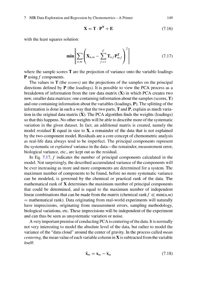
where the sample scores T are the projection of variance onto the variable loadings
P using f components.
The values in T (the scores) are the projections of the samples on the principal
directions defined by P (the loadings). It is possible to view the PCA process as a
breakdown of information from the raw data matrix (X) in which PCA creates two
new, smaller data matrices: one containing information about the samples (scores, T)
and one containing information about the variables (loadings, P). The splitting of the
information is done in such a way that the two parts, T and P, explain as much variation in the original data matrix (X). The PCA algorithm finds the weights (loadings)
so that this happens. No other weights will be able to describe more of the systematic
variation in the given dataset. In fact, an additional matrix is created, namely the
model residual E equal in size to X, a remainder of the data that is not explained
by the two-component model. Residuals are a core concept of chemometric analysis
as real-life data always tend to be imperfect. The principal components represent
the systematic or explained variance in the data—the remainder, measurement error,
biological variance, etc., are kept out as the residual.
In Eq. 7.17, f indicates the number of principal components calculated in the
model. Not surprisingly, the described accumulated variance of the components will
be ever increasing as more and more components are determined for a system. The
maximum number of components to be found, before no more systematic variance
can be modeled, is governed by the chemical or practical rank of the data. The
mathematical rank of X determines the maximum number of principal components
that could be determined, and is equal to the maximum number of independent
linear combinations that can be made from the matrix (chemical rank f min(n,m)
= mathematical rank). Data originating from real-world experiments will naturally
have imprecisions, originating from measurement errors, sampling methodology,
biological variations, etc. These imprecisions will be independent of the experiment
and can thus be seen as unsystematic variation or noise.
A very important premise of conducting PCA is centering of the data. It is normally
not very interesting to model the absolute level of the data, but rather to model the
variance of the “data cloud” around the center of gravity. In the process called mean
centering, the mean value of each variable column in X is subtracted from the variable
itself:
ˆ
x m = x m − x m
(7.18)
149
X = T · P
T
+ E
(7.16)
with the least squares solution:
min
n,m
⎛
⎝ X n,m −
F
f =1
T n,f P
T
m,f
⎞
⎠
2
(7.17)
where the sample scores T are the projection of variance onto the variable loadings
P using f components.
The values in T (the scores) are the projections of the samples on the principal
directions defined by P (the loadings). It is possible to view the PCA process as a
breakdown of information from the raw data matrix (X) in which PCA creates two
new, smaller data matrices: one containing information about the samples (scores, T)
and one containing information about the variables (loadings, P). The splitting of the
information is done in such a way that the two parts, T and P, explain as much variation in the original data matrix (X). The PCA algorithm finds the weights (loadings)
so that this happens. No other weights will be able to describe more of the systematic
variation in the given dataset. In fact, an additional matrix is created, namely the
model residual E equal in size to X, a remainder of the data that is not explained
by the two-component model. Residuals are a core concept of chemometric analysis
as real-life data always tend to be imperfect. The principal components represent
the systematic or explained variance in the data—the remainder, measurement error,
biological variance, etc., are kept out as the residual.
In Eq. 7.17, f indicates the number of principal components calculated in the
model. Not surprisingly, the described accumulated variance of the components will
be ever increasing as more and more components are determined for a system. The
maximum number of components to be found, before no more systematic variance
can be modeled, is governed by the chemical or practical rank of the data. The
mathematical rank of X determines the maximum number of principal components
that could be determined, and is equal to the maximum number of independent
linear combinations that can be made from the matrix (chemical rank f min(n,m)
= mathematical rank). Data originating from real-world experiments will naturally
have imprecisions, originating from measurement errors, sampling methodology,
biological variations, etc. These imprecisions will be independent of the experiment
and can thus be seen as unsystematic variation or noise.
A very important premise of conducting PCA is centering of the data. It is normally
not very interesting to model the absolute level of the data, but rather to model the
variance of the “data cloud” around the center of gravity. In the process called mean
centering, the mean value of each variable column in X is subtracted from the variable
itself:
ˆ
x m = x m − x m
(7.18)