

148
K. M. Sørensen et al.
Variable 2
Variable 2
Variable 2
Variable 2
Factor 1
Factor 1
Factor 1
Factor 2s
a
b
c
d
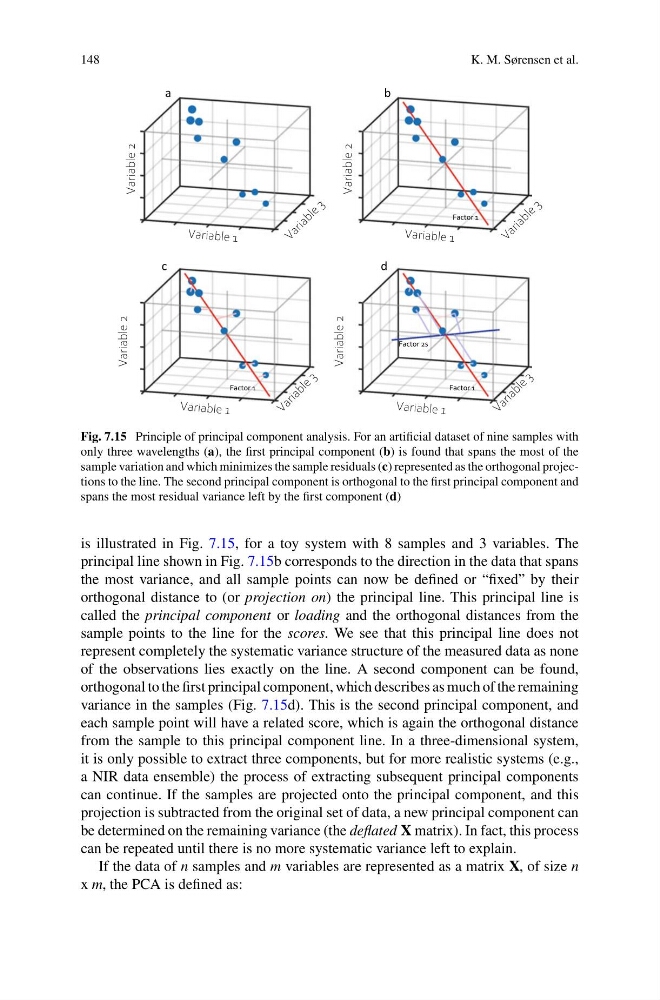
Fig. 7.15 Principle of principal component analysis. For an artificial dataset of nine samples with
only three wavelengths (a), the first principal component (b) is found that spans the most of the
sample variation and which minimizes the sample residuals (c) represented as the orthogonal projections to the line. The second principal component is orthogonal to the first principal component and
spans the most residual variance left by the first component (d)
is illustrated in Fig. 7.15, for a toy system with 8 samples and 3 variables. The
principal line shown in Fig. 7.15b corresponds to the direction in the data that spans
the most variance, and all sample points can now be defined or “fixed” by their
orthogonal distance to (or projection on) the principal line. This principal line is
called the principal component or loading and the orthogonal distances from the
sample points to the line for the scores. We see that this principal line does not
represent completely the systematic variance structure of the measured data as none
of the observations lies exactly on the line. A second component can be found,
orthogonal to the first principal component, which describes as much of the remaining
variance in the samples (Fig. 7.15d). This is the second principal component, and
each sample point will have a related score, which is again the orthogonal distance
from the sample to this principal component line. In a three-dimensional system,
it is only possible to extract three components, but for more realistic systems (e.g.,
a NIR data ensemble) the process of extracting subsequent principal components
can continue. If the samples are projected onto the principal component, and this
projection is subtracted from the original set of data, a new principal component can
be determined on the remaining variance (the deflated X matrix). In fact, this process
can be repeated until there is no more systematic variance left to explain.
If the data of n samples and m variables are represented as a matrix X, of size n
x m, the PCA is defined as:
K. M. Sørensen et al.
Variable 2
Variable 2
Variable 2
Variable 2
Factor 1
Factor 1
Factor 1
Factor 2s
a
b
c
d
Fig. 7.15 Principle of principal component analysis. For an artificial dataset of nine samples with
only three wavelengths (a), the first principal component (b) is found that spans the most of the
sample variation and which minimizes the sample residuals (c) represented as the orthogonal projections to the line. The second principal component is orthogonal to the first principal component and
spans the most residual variance left by the first component (d)
is illustrated in Fig. 7.15, for a toy system with 8 samples and 3 variables. The
principal line shown in Fig. 7.15b corresponds to the direction in the data that spans
the most variance, and all sample points can now be defined or “fixed” by their
orthogonal distance to (or projection on) the principal line. This principal line is
called the principal component or loading and the orthogonal distances from the
sample points to the line for the scores. We see that this principal line does not
represent completely the systematic variance structure of the measured data as none
of the observations lies exactly on the line. A second component can be found,
orthogonal to the first principal component, which describes as much of the remaining
variance in the samples (Fig. 7.15d). This is the second principal component, and
each sample point will have a related score, which is again the orthogonal distance
from the sample to this principal component line. In a three-dimensional system,
it is only possible to extract three components, but for more realistic systems (e.g.,
a NIR data ensemble) the process of extracting subsequent principal components
can continue. If the samples are projected onto the principal component, and this
projection is subtracted from the original set of data, a new principal component can
be determined on the remaining variance (the deflated X matrix). In fact, this process
can be repeated until there is no more systematic variance left to explain.
If the data of n samples and m variables are represented as a matrix X, of size n
x m, the PCA is defined as: