

118
M. A. Czarnecki and S. Morita
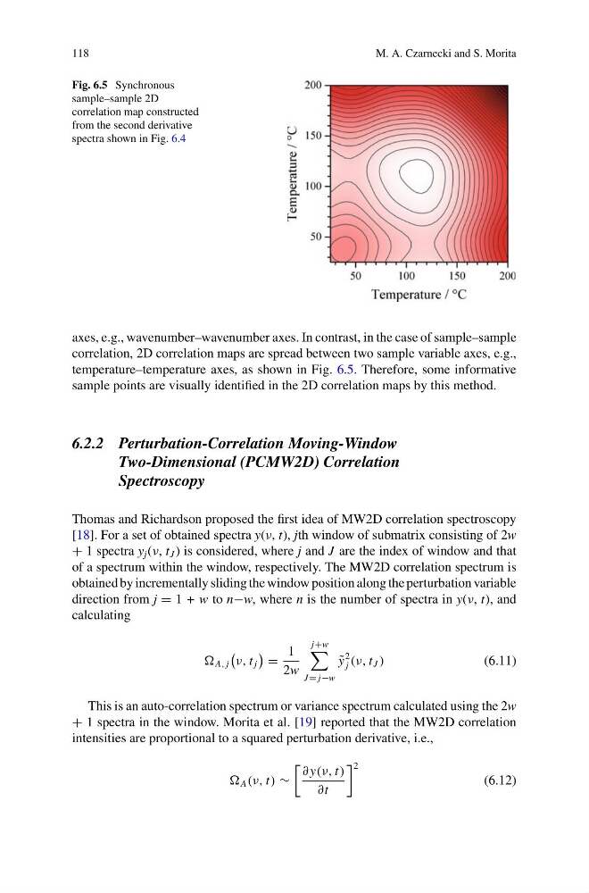
Fig. 6.5 Synchronous
sample–sample 2D
correlation map constructed
from the second derivative
spectra shown in Fig. 6.4
axes, e.g., wavenumber–wavenumber axes. In contrast, in the case of sample–sample
correlation, 2D correlation maps are spread between two sample variable axes, e.g.,
temperature–temperature axes, as shown in Fig. 6.5. Therefore, some informative
sample points are visually identified in the 2D correlation maps by this method.
6.2.2 Perturbation-Correlation Moving-Window
Two-Dimensional (PCMW2D) Correlation
Spectroscopy
Thomas and Richardson proposed the first idea of MW2D correlation spectroscopy
[18]. For a set of obtained spectra y(ν, t), jth window of submatrix consisting of 2w
+ 1 spectra y j (ν, t J ) is considered, where j and J are the index of window and that
of a spectrum within the window, respectively. The MW2D correlation spectrum is
obtained by incrementally sliding the window position along the perturbation variable
direction from j = 1 + w to n−w, where n is the number of spectra in y(ν, t), and
calculating
A, j
ν, t j
=
1
2w
j+w
J = j−w
˜
y
2
j (ν, t J )
(6.11)
This is an auto-correlation spectrum or variance spectrum calculated using the 2w
+ 1 spectra in the window. Morita et al. [19] reported that the MW2D correlation
intensities are proportional to a squared perturbation derivative, i.e.,
A (ν, t) ∼
∂ y(ν, t)
∂t
2
(6.12)
M. A. Czarnecki and S. Morita
Fig. 6.5 Synchronous
sample–sample 2D
correlation map constructed
from the second derivative
spectra shown in Fig. 6.4
axes, e.g., wavenumber–wavenumber axes. In contrast, in the case of sample–sample
correlation, 2D correlation maps are spread between two sample variable axes, e.g.,
temperature–temperature axes, as shown in Fig. 6.5. Therefore, some informative
sample points are visually identified in the 2D correlation maps by this method.
6.2.2 Perturbation-Correlation Moving-Window
Two-Dimensional (PCMW2D) Correlation
Spectroscopy
Thomas and Richardson proposed the first idea of MW2D correlation spectroscopy
[18]. For a set of obtained spectra y(ν, t), jth window of submatrix consisting of 2w
+ 1 spectra y j (ν, t J ) is considered, where j and J are the index of window and that
of a spectrum within the window, respectively. The MW2D correlation spectrum is
obtained by incrementally sliding the window position along the perturbation variable
direction from j = 1 + w to n−w, where n is the number of spectra in y(ν, t), and
calculating
A, j
ν, t j
=
1
2w
j+w
J = j−w
˜
y
2
j (ν, t J )
(6.11)
This is an auto-correlation spectrum or variance spectrum calculated using the 2w
+ 1 spectra in the window. Morita et al. [19] reported that the MW2D correlation
intensities are proportional to a squared perturbation derivative, i.e.,
A (ν, t) ∼
∂ y(ν, t)
∂t
2
(6.12)