

6 Two-Dimensional Correlation Spectroscopy
117
6.2 New Developments in Two-Dimensional Correlation
Spectroscopy
6.2.1 Sample–Sample Correlation Spectroscopy
For the last two decades or so, several new ideas regarding 2DCOS have been
proposed such as sample–sample (SS), moving-window two-dimensional (MW2D)
and perturbation-correlation moving-window two-dimensional (PCMW2D). Here,
SS, MW2D and PCMW2D methods will be outlined. The first idea of sample–sample
correlation, i.e., opposite to conventional variable–variable correlation, was proposed
by Zimba [14], and this idea was subsequently refined by Šaši´ c et al. [15, 16]. As
given in Eq. (4), the conventional synchronous 2D correlation spectrum
ν i , ν j
is
calculated as a covariance matrix of y(ν, t). The synchronous sample–sample correlation ( SS ) is given as a covariance matrix of transposed y(ν, t) matrix, and the
asynchronous sample–sample correlation ( SS ) is calculated as:
SS (t k , t l ) =
1
m − 1
˜
y(ν, t k ) · ˜
y(ν, t l )
T
(6.9)
Ψ SS (t k , t l ) =
1
m − 1
˜
y(ν, t k ) · M · ˜
y(ν, t l )
T
(6.10)
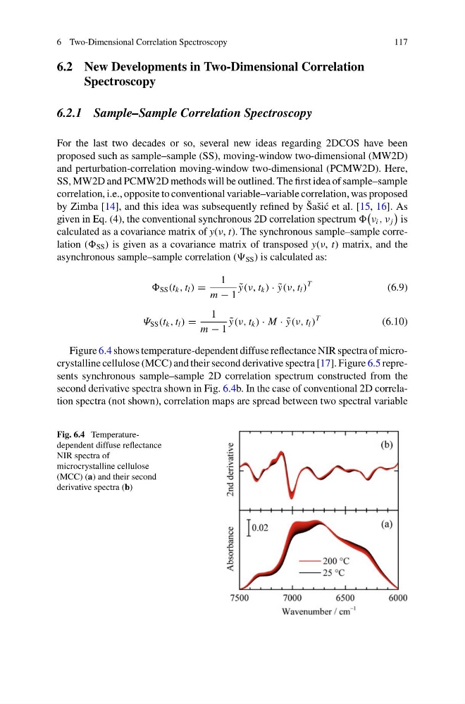
Figure 6.4 shows temperature-dependent diffuse reflectance NIR spectra of microcrystalline cellulose (MCC) and their second derivative spectra [17]. Figure 6.5 represents synchronous sample–sample 2D correlation spectrum constructed from the
second derivative spectra shown in Fig. 6.4b. In the case of conventional 2D correlation spectra (not shown), correlation maps are spread between two spectral variable
Fig. 6.4 Temperaturedependent diffuse reflectance
NIR spectra of
microcrystalline cellulose
(MCC) (a) and their second
derivative spectra (b)
117
6.2 New Developments in Two-Dimensional Correlation
Spectroscopy
6.2.1 Sample–Sample Correlation Spectroscopy
For the last two decades or so, several new ideas regarding 2DCOS have been
proposed such as sample–sample (SS), moving-window two-dimensional (MW2D)
and perturbation-correlation moving-window two-dimensional (PCMW2D). Here,
SS, MW2D and PCMW2D methods will be outlined. The first idea of sample–sample
correlation, i.e., opposite to conventional variable–variable correlation, was proposed
by Zimba [14], and this idea was subsequently refined by Šaši´ c et al. [15, 16]. As
given in Eq. (4), the conventional synchronous 2D correlation spectrum
ν i , ν j
is
calculated as a covariance matrix of y(ν, t). The synchronous sample–sample correlation ( SS ) is given as a covariance matrix of transposed y(ν, t) matrix, and the
asynchronous sample–sample correlation ( SS ) is calculated as:
SS (t k , t l ) =
1
m − 1
˜
y(ν, t k ) · ˜
y(ν, t l )
T
(6.9)
Ψ SS (t k , t l ) =
1
m − 1
˜
y(ν, t k ) · M · ˜
y(ν, t l )
T
(6.10)
Figure 6.4 shows temperature-dependent diffuse reflectance NIR spectra of microcrystalline cellulose (MCC) and their second derivative spectra [17]. Figure 6.5 represents synchronous sample–sample 2D correlation spectrum constructed from the
second derivative spectra shown in Fig. 6.4b. In the case of conventional 2D correlation spectra (not shown), correlation maps are spread between two spectral variable
Fig. 6.4 Temperaturedependent diffuse reflectance
NIR spectra of
microcrystalline cellulose
(MCC) (a) and their second
derivative spectra (b)