

114
M. A. Czarnecki and S. Morita
sample composition, temperature, pressure, pH and so on. Each kind of perturbation yields unique information about studied system. It is also important to apply an
appropriate probe to successfully monitor the perturbation-induced changes in the
studied system.
As mentioned before, the generalized 2DCOS permits for hetero-correlation of
two unlike types of data; however, both data sets have to be recorded under the
same perturbation values. If ˜
y and ˜
u are the dynamic spectra from two different
experiments, then the synchronous and asynchronous hetero-correlation spectra are
expressed:
ν i , μ j
=
1
n − 1
˜
y(ν i , t)
T
· ˜
u
μ j , t
(6.7)
ν i , μ j
=
1
n − 1
˜
y(ν i , t)
T
· M · ˜
u
μ j , t
(6.8)
The properties of the synchronous and asynchronous spectra were explained by
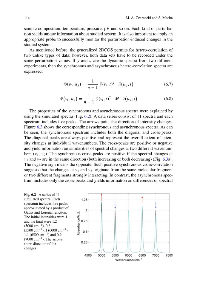
using the simulated spectra (Fig. 6.2). A data series consist of 11 spectra and each
spectrum includes five peaks. The arrows point the direction of intensity changes.
Figure 6.3 shows the corresponding synchronous and asynchronous spectra. As can
be seen, the synchronous spectrum includes both the diagonal and cross-peaks.
The diagonal peaks are always positive and represent the overall extent of intensity changes at individual wavenumbers. The cross-peaks are positive or negative
and yield information on similarities of spectral changes at two different wavenumbers (ν 1 , ν 2 ). The synchronous cross-peaks are positive if the spectral changes at
ν 1 and ν 2 are in the same direction (both increasing or both decreasing) (Fig. 6.3a).
The negative sign means the opposite. Such positive synchronous cross-correlation
suggests that the changes at ν 1 and ν 2 originate from the same molecular fragment
or two different fragments strongly interacting. In contrast, the asynchronous spectrum includes only the cross-peaks and yields information on differences of spectral
Fig. 6.2 A series of 11
simulated spectra. Each
spectrum includes five peaks
approximated by a product of
Gauss and Lorentz function.
The initial intensities were 1
and the final were 1.2
(5000 cm −1 ), 0.8
(5500 cm −1 ), 1 (6000 cm −1 ),
1.1 (6500 cm −1 ) and 0.9
(7000 cm −1 ). The arrows
show direction of the
changes
M. A. Czarnecki and S. Morita
sample composition, temperature, pressure, pH and so on. Each kind of perturbation yields unique information about studied system. It is also important to apply an
appropriate probe to successfully monitor the perturbation-induced changes in the
studied system.
As mentioned before, the generalized 2DCOS permits for hetero-correlation of
two unlike types of data; however, both data sets have to be recorded under the
same perturbation values. If ˜
y and ˜
u are the dynamic spectra from two different
experiments, then the synchronous and asynchronous hetero-correlation spectra are
expressed:
ν i , μ j
=
1
n − 1
˜
y(ν i , t)
T
· ˜
u
μ j , t
(6.7)
ν i , μ j
=
1
n − 1
˜
y(ν i , t)
T
· M · ˜
u
μ j , t
(6.8)
The properties of the synchronous and asynchronous spectra were explained by
using the simulated spectra (Fig. 6.2). A data series consist of 11 spectra and each
spectrum includes five peaks. The arrows point the direction of intensity changes.
Figure 6.3 shows the corresponding synchronous and asynchronous spectra. As can
be seen, the synchronous spectrum includes both the diagonal and cross-peaks.
The diagonal peaks are always positive and represent the overall extent of intensity changes at individual wavenumbers. The cross-peaks are positive or negative
and yield information on similarities of spectral changes at two different wavenumbers (ν 1 , ν 2 ). The synchronous cross-peaks are positive if the spectral changes at
ν 1 and ν 2 are in the same direction (both increasing or both decreasing) (Fig. 6.3a).
The negative sign means the opposite. Such positive synchronous cross-correlation
suggests that the changes at ν 1 and ν 2 originate from the same molecular fragment
or two different fragments strongly interacting. In contrast, the asynchronous spectrum includes only the cross-peaks and yields information on differences of spectral
Fig. 6.2 A series of 11
simulated spectra. Each
spectrum includes five peaks
approximated by a product of
Gauss and Lorentz function.
The initial intensities were 1
and the final were 1.2
(5000 cm −1 ), 0.8
(5500 cm −1 ), 1 (6000 cm −1 ),
1.1 (6500 cm −1 ) and 0.9
(7000 cm −1 ). The arrows
show direction of the
changes