

6 Two-Dimensional Correlation Spectroscopy
113
⎡
⎢
⎢
⎢
⎢
⎢
⎣
y(ν 1 , t 1 ) y(ν 2 , t 1 ) · · · y(ν m , t 1 )
y(ν 1 , t 2 ) y(ν 2 , t 2 ) · · · y(ν m , t 2 )
y(ν 1 , t 3 ) y(ν 2 , t 3 ) · · · y(ν m , t 3 )
· · ·
· · · · · ·
· · ·
y(ν 1 , t n ) y(ν 2 , t n ) · · · y(ν m , t n )
⎤
⎥
⎥
⎥
⎥
⎥
⎦
(6.1)
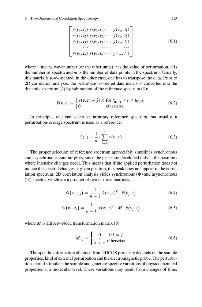
where ν means wavenumber (or the other units), t is the value of perturbation, n is
the number of spectra and m is the number of data points in the spectrum. Usually,
this matrix is row-oriented; in the other case, one has to transpose the data. Prior to
2D correlation analysis, the perturbation-ordered data matrix is converted into the
dynamic spectrum ( ˜
y) by subtraction of the reference spectrum ( ˆ
y):
˜
y(ν, t) =
y(ν, t) − ˆ
y(ν) for t min ≤ t ≤ t max
0
otherwise
(6.2)
In principle, one can select an arbitrary reference spectrum, but usually, a
perturbation-average spectrum is used as a reference:
ˆ
y(ν) =
1
n
·
n
i=1
y(ν, t i )
(6.3)
The proper selection of reference spectrum appreciably simplifies synchronous
and asynchronous contour plots, since the peaks are developed only at the positions
where intensity changes occur. This means that if the applied perturbation does not
induce the spectral changes at given position, this peak does not appear in the correlation spectrum. 2D correlation analysis yields synchronous () and asynchronous
() spectra, which are a product of two or three matrices:
ν i , ν j
=
1
n − 1
˜
y(ν i , t)
T
· ˜
y
ν j , t
(6.4)
ν i , ν j
=
1
n − 1
˜
y(ν i , t)
T
· M · ˜
y
ν j , t
(6.5)
where M is Hilbert–Noda transformation matrix [8]:
M i, j =
0
ifi = j
1
π·( j−i)
otherwise
(6.6)
The specific information obtained from 2DCOS primarily depends on the sample
properties, kind of external perturbation and the electromagnetic probe. The perturbation should stimulate the sample and generate specific variations of physicochemical
properties at a molecular level. These variations may result from changes of time,
113
⎡
⎢
⎢
⎢
⎢
⎢
⎣
y(ν 1 , t 1 ) y(ν 2 , t 1 ) · · · y(ν m , t 1 )
y(ν 1 , t 2 ) y(ν 2 , t 2 ) · · · y(ν m , t 2 )
y(ν 1 , t 3 ) y(ν 2 , t 3 ) · · · y(ν m , t 3 )
· · ·
· · · · · ·
· · ·
y(ν 1 , t n ) y(ν 2 , t n ) · · · y(ν m , t n )
⎤
⎥
⎥
⎥
⎥
⎥
⎦
(6.1)
where ν means wavenumber (or the other units), t is the value of perturbation, n is
the number of spectra and m is the number of data points in the spectrum. Usually,
this matrix is row-oriented; in the other case, one has to transpose the data. Prior to
2D correlation analysis, the perturbation-ordered data matrix is converted into the
dynamic spectrum ( ˜
y) by subtraction of the reference spectrum ( ˆ
y):
˜
y(ν, t) =
y(ν, t) − ˆ
y(ν) for t min ≤ t ≤ t max
0
otherwise
(6.2)
In principle, one can select an arbitrary reference spectrum, but usually, a
perturbation-average spectrum is used as a reference:
ˆ
y(ν) =
1
n
·
n
i=1
y(ν, t i )
(6.3)
The proper selection of reference spectrum appreciably simplifies synchronous
and asynchronous contour plots, since the peaks are developed only at the positions
where intensity changes occur. This means that if the applied perturbation does not
induce the spectral changes at given position, this peak does not appear in the correlation spectrum. 2D correlation analysis yields synchronous () and asynchronous
() spectra, which are a product of two or three matrices:
ν i , ν j
=
1
n − 1
˜
y(ν i , t)
T
· ˜
y
ν j , t
(6.4)
ν i , ν j
=
1
n − 1
˜
y(ν i , t)
T
· M · ˜
y
ν j , t
(6.5)
where M is Hilbert–Noda transformation matrix [8]:
M i, j =
0
ifi = j
1
π·( j−i)
otherwise
(6.6)
The specific information obtained from 2DCOS primarily depends on the sample
properties, kind of external perturbation and the electromagnetic probe. The perturbation should stimulate the sample and generate specific variations of physicochemical
properties at a molecular level. These variations may result from changes of time,