

104
K. B. Be´ c et al.
5.5.2 Grid-Based Approaches
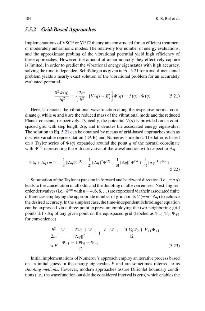
Implementations of VSCF or VPT2 theory are constructed for an efficient treatment
of moderately anharmonic modes. The relatively low number of energy evaluations,
and the approximate probing of the vibrational potential yield high efficiency of
these approaches. However, the amount of anharmonicity they effectively capture
is limited. In order to predict the vibrational energy eigenstates with high accuracy,
solving the time-independent Schrödinger as given in Eq. 5.21 for a one-dimensional
problem yields a nearly exact solution of the vibrational problem for an accurately
evaluated potential.
∂
2
(q)
∂q 2 =
2m
2 ·
V (q) − E
(q) = f (q) · (q)
(5.21)
Here, denotes the vibrational wavefunction along the respective normal coordinate q, while m and are the reduced mass of the vibrational mode and the reduced
Planck constant, respectively. Typically, the potential V (q) is provided on an equispaced grid with step length q, and E denotes the associated energy eigenvalue.
The solution to Eq. 5.21 can be obtained by means of grid-based approaches such as
discrete variable representation (DVR) and Numerov’s method. The latter is based
on a Taylor series of (q) expanded around the point q of the normal coordinate
with
(n) representing the n-th derivative of the wavefunction with respect to q:
(q + q) = +
1
1!
q
(1) +
1
2!
q
2
(2) +
1
3!
q
3
(3) +
1
4!
q
4
(4) + · · ·
(5.22)
Summation of the Taylor expansion in forward and backward direction (i.e., ±q)
leads to the cancellation of all odd, and the doubling of all even entries. Next, higherorder derivatives (i.e.,
(n) with n = 4, 6, 8, …) are expressed via their associated finite
differences employing the appropriate number of grid points V (±m · q) to achieve
the desired accuracy. In the simplest case, the time-independent Schrödinger equation
can be expressed via a three-point expression employing the two neighboring grid
points ±1 · q of any given point on the equispaced grid (labeled as −1, 0 , , +1
for convenience)
−
2
2m
·
−1 − 2 0 + +1
q
2
+
V −1 −1 + 10V 0 0 + V +1 +1
12
≈ E ·
−1 + 10 0 + +1
12
(5.23)
Initial implementations of Numerov’s approach employ an iterative process based
on an initial guess in the energy eigenvalue E and are sometimes referred to as
shooting methods. However, modern approaches assure Dirichlet boundary conditions (i.e., the wavefunction outside the considered interval is zero) which enables the
K. B. Be´ c et al.
5.5.2 Grid-Based Approaches
Implementations of VSCF or VPT2 theory are constructed for an efficient treatment
of moderately anharmonic modes. The relatively low number of energy evaluations,
and the approximate probing of the vibrational potential yield high efficiency of
these approaches. However, the amount of anharmonicity they effectively capture
is limited. In order to predict the vibrational energy eigenstates with high accuracy,
solving the time-independent Schrödinger as given in Eq. 5.21 for a one-dimensional
problem yields a nearly exact solution of the vibrational problem for an accurately
evaluated potential.
∂
2
(q)
∂q 2 =
2m
2 ·
V (q) − E
(q) = f (q) · (q)
(5.21)
Here, denotes the vibrational wavefunction along the respective normal coordinate q, while m and are the reduced mass of the vibrational mode and the reduced
Planck constant, respectively. Typically, the potential V (q) is provided on an equispaced grid with step length q, and E denotes the associated energy eigenvalue.
The solution to Eq. 5.21 can be obtained by means of grid-based approaches such as
discrete variable representation (DVR) and Numerov’s method. The latter is based
on a Taylor series of (q) expanded around the point q of the normal coordinate
with
(n) representing the n-th derivative of the wavefunction with respect to q:
(q + q) = +
1
1!
q
(1) +
1
2!
q
2
(2) +
1
3!
q
3
(3) +
1
4!
q
4
(4) + · · ·
(5.22)
Summation of the Taylor expansion in forward and backward direction (i.e., ±q)
leads to the cancellation of all odd, and the doubling of all even entries. Next, higherorder derivatives (i.e.,
(n) with n = 4, 6, 8, …) are expressed via their associated finite
differences employing the appropriate number of grid points V (±m · q) to achieve
the desired accuracy. In the simplest case, the time-independent Schrödinger equation
can be expressed via a three-point expression employing the two neighboring grid
points ±1 · q of any given point on the equispaced grid (labeled as −1, 0 , , +1
for convenience)
−
2
2m
·
−1 − 2 0 + +1
q
2
+
V −1 −1 + 10V 0 0 + V +1 +1
12
≈ E ·
−1 + 10 0 + +1
12
(5.23)
Initial implementations of Numerov’s approach employ an iterative process based
on an initial guess in the energy eigenvalue E and are sometimes referred to as
shooting methods. However, modern approaches assure Dirichlet boundary conditions (i.e., the wavefunction outside the considered interval is zero) which enables the