

2.1 Holographic Microscopy for the Study of Phase, Diffusive …
71
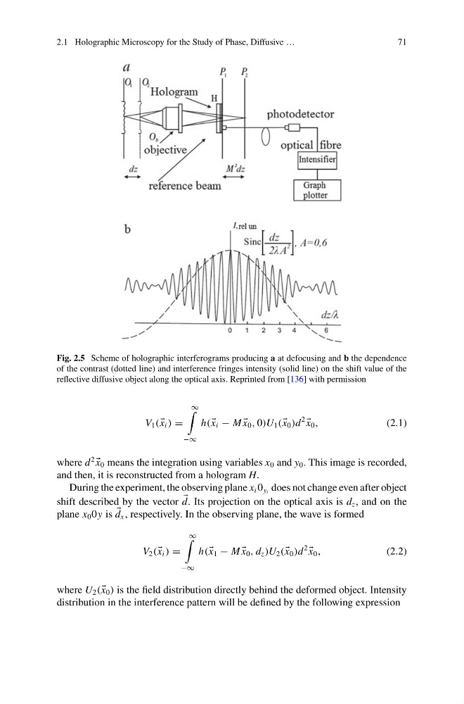
Fig. 2.5 Scheme of holographic interferograms producing a at defocusing and b the dependence
of the contrast (dotted line) and interference fringes intensity (solid line) on the shift value of the
reflective diffusive object along the optical axis. Reprinted from [136] with permission
V 1 ( x i ) =
∞
−∞
h( x i − M
x 0 , 0)U 1 ( x 0 )d
2
x 0 ,
(2.1)
where d
2
x 0 means the integration using variables x 0 and y 0 . This image is recorded,
and then, it is reconstructed from a hologram H.
During the experiment, the observing plane x i 0 y i does not change even after object
shift described by the vector
d. Its projection on the optical axis is d z , and on the
plane x 0 0y is
d x , respectively. In the observing plane, the wave is formed
V 2 ( x i ) =
∞
−∞
h( x 1 − M
x 0 , d z )U 2 ( x 0 )d
2
x 0 ,
(2.2)
where U 2 ( x 0 ) is the field distribution directly behind the deformed object. Intensity
distribution in the interference pattern will be defined by the following expression
71
Fig. 2.5 Scheme of holographic interferograms producing a at defocusing and b the dependence
of the contrast (dotted line) and interference fringes intensity (solid line) on the shift value of the
reflective diffusive object along the optical axis. Reprinted from [136] with permission
V 1 ( x i ) =
∞
−∞
h( x i − M
x 0 , 0)U 1 ( x 0 )d
2
x 0 ,
(2.1)
where d
2
x 0 means the integration using variables x 0 and y 0 . This image is recorded,
and then, it is reconstructed from a hologram H.
During the experiment, the observing plane x i 0 y i does not change even after object
shift described by the vector
d. Its projection on the optical axis is d z , and on the
plane x 0 0y is
d x , respectively. In the observing plane, the wave is formed
V 2 ( x i ) =
∞
−∞
h( x 1 − M
x 0 , d z )U 2 ( x 0 )d
2
x 0 ,
(2.2)
where U 2 ( x 0 ) is the field distribution directly behind the deformed object. Intensity
distribution in the interference pattern will be defined by the following expression