

18
1 Resonance Methods for Increasing Sensitivity of Interferometry …
As it can be seen from Fig. 1.7 from the whole generating end area of 2 × 3 mm
2
(pumping energy is 0.04 J), spatial coherence area (0.2 level) takes 1.3 × 1.3 mm
2 . If
pumping energy is E = 0.03 J, then this area is narrowed to 0.8 mm
2 (the comparison
is given for one-axis points, Fig. 1.7c, g). Spatial coherence function contour had
one maximum. The coherence area sizes from pulse to pulse have not been changed
(under pumping energy E = 0.04 J and dye concentration corresponding to absorption
constant of 12 cm
−1 for λ = 347.2 nm). Dependence of this area on the concentration
(in the studied concentrations interval of corresponding to absorption constants of
10–18 cm
−1 for λ = 347.2 nm) under constant level of pumping energy of 0.04 J was
weakly evident. At the same time, we could observe strong dependence of coherence
area sizes in the direction of pumping pulse propagation on pumping energy. When
the pumping energy was E = 0.04–0.05 J, coherence area size was the largest and
formed 1.3 mm, in the case when pumping energy was 0.01 J, coherence area size
was decreasing to 0.2 mm. In Fig. 1.7, the dotted line shows intensity distribution
in the reconstructed image of diffusive screen, which is also the characteristics of
coherence, because, namely it characterizes the quantity of coherent light emitted
by laser end points. It seems that asymmetry of the initial intensity distribution on
the laser end (see Fig. 1.7a, b, e, f—solid line) is provided by unsteady optical
inhomogeneity. It appears under transverse, concerning cavity axis, pumping pulse
and also under the presence of the Fabry–Perot interferometer in the resonator. Along
with the determination of spatial coherence function of dye laser, the comparison of
values |γ | for one of the generation pulses was carried out. This comparison was made
using two different methods: microphotometry method and holographic method. The
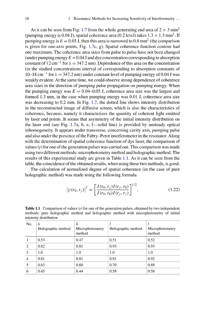
results of this experimental study are given in Table 1.1. As it can be seen from the
table, the coincidence of the obtained results, when using these two methods, is good.
The calculation of normalized degree of spatial coherence (in the case of pure
holographic method) was made using the following formula
γ (r 0 , r j )
2 =
I (r 0 , r j )I (r j , r 0 )
I (r 0 , r 0 )I (r j , r j )
1/2
,
(1.22)
Table 1.1 Comparison of values |γ | for one of the generation pulses, obtained by two independent
methods: pure holographic method and holographic method with microphotometry of initial
intensity distribution
No. h
Holographic method
h
Microphotometry
method
l
Holographic method
l
Microphotometry
method
1
0.53
0.47
0.51
0.52
2
0.82
0.81
0.93
0.93
3
1.0
1.0
1.0
1.0
4
0.81
0.81
0.91
0.92
5
0.63
0.60
0.70
0.69
6
0.45
0.44
0.58
0.58
1 Resonance Methods for Increasing Sensitivity of Interferometry …
As it can be seen from Fig. 1.7 from the whole generating end area of 2 × 3 mm
2
(pumping energy is 0.04 J), spatial coherence area (0.2 level) takes 1.3 × 1.3 mm
2 . If
pumping energy is E = 0.03 J, then this area is narrowed to 0.8 mm
2 (the comparison
is given for one-axis points, Fig. 1.7c, g). Spatial coherence function contour had
one maximum. The coherence area sizes from pulse to pulse have not been changed
(under pumping energy E = 0.04 J and dye concentration corresponding to absorption
constant of 12 cm
−1 for λ = 347.2 nm). Dependence of this area on the concentration
(in the studied concentrations interval of corresponding to absorption constants of
10–18 cm
−1 for λ = 347.2 nm) under constant level of pumping energy of 0.04 J was
weakly evident. At the same time, we could observe strong dependence of coherence
area sizes in the direction of pumping pulse propagation on pumping energy. When
the pumping energy was E = 0.04–0.05 J, coherence area size was the largest and
formed 1.3 mm, in the case when pumping energy was 0.01 J, coherence area size
was decreasing to 0.2 mm. In Fig. 1.7, the dotted line shows intensity distribution
in the reconstructed image of diffusive screen, which is also the characteristics of
coherence, because, namely it characterizes the quantity of coherent light emitted
by laser end points. It seems that asymmetry of the initial intensity distribution on
the laser end (see Fig. 1.7a, b, e, f—solid line) is provided by unsteady optical
inhomogeneity. It appears under transverse, concerning cavity axis, pumping pulse
and also under the presence of the Fabry–Perot interferometer in the resonator. Along
with the determination of spatial coherence function of dye laser, the comparison of
values |γ | for one of the generation pulses was carried out. This comparison was made
using two different methods: microphotometry method and holographic method. The
results of this experimental study are given in Table 1.1. As it can be seen from the
table, the coincidence of the obtained results, when using these two methods, is good.
The calculation of normalized degree of spatial coherence (in the case of pure
holographic method) was made using the following formula
γ (r 0 , r j )
2 =
I (r 0 , r j )I (r j , r 0 )
I (r 0 , r 0 )I (r j , r j )
1/2
,
(1.22)
Table 1.1 Comparison of values |γ | for one of the generation pulses, obtained by two independent
methods: pure holographic method and holographic method with microphotometry of initial
intensity distribution
No. h
Holographic method
h
Microphotometry
method
l
Holographic method
l
Microphotometry
method
1
0.53
0.47
0.51
0.52
2
0.82
0.81
0.93
0.93
3
1.0
1.0
1.0
1.0
4
0.81
0.81
0.91
0.92
5
0.63
0.60
0.70
0.69
6
0.45
0.44
0.58
0.58