

1.2 Spatial Coherence of Rhodamine 6G Laser Radiation …
13
where constant C 2 is directly detected from |γ (0)|
2
= 1.
Thus, for the calculation of the average distribution |˜ y(x)|
2 , it is necessary to
determine experimentally the value of the integral intensity I i (r) and the intensity
distribution on the laser edge I 0 (r). Further calculations can be made, for example,
using computer or in the analytical form using function approximation I i (r) and
I 0 (r).
1.2.2 Measuring Spatial Coherence of 6G Rhodamine Laser
Pumping by Interference and Holographic Methods:
Holographic, Holographic with Microphotometry
of Initial Intensity Distribution and Integral
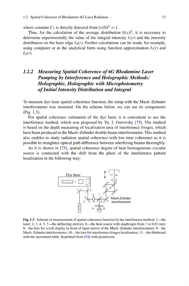
To measure dye laser spatial coherence function, the setup with the Mach–Zehnder
interferometer was mounted. On the scheme below, we can see its components
(Fig. 1.3).
For spatial coherence estimation of the dye laser, it is convenient to use the
interference method, which was proposed by Yu. I. Ostrovsky [75]. The method
is based on the depth measuring of localization area of interference fringes, which
have been produced in the Mach–Zehnder double-beam interferometer. This method
also enables to study radiation spatial coherence with low time coherence as it is
possible to straighten optical path difference between interfering beams thoroughly.
As it is shown in [75], spatial coherence degree of heat homogeneous circular
source is connected with the shift from the plane of the interference pattern
localization in the following way:
Fig. 1.3 Scheme of measurement of spatial coherence function by the interference method: 1—the
laser; 2, 3, 4, 5, 7—the deflecting mirrors; 6—the heat source with diaphragm from 1 to 0.01 mm;
8—the lens for scroll display in front of input mirror of the Mach–Zehnder interferometer; 9—the
Mach–Zehnder interferometer; 10—the lens for interference fringes localization; 11—the filmboard
with the movement table. Reprinted from [54] with permission
13
where constant C 2 is directly detected from |γ (0)|
2
= 1.
Thus, for the calculation of the average distribution |˜ y(x)|
2 , it is necessary to
determine experimentally the value of the integral intensity I i (r) and the intensity
distribution on the laser edge I 0 (r). Further calculations can be made, for example,
using computer or in the analytical form using function approximation I i (r) and
I 0 (r).
1.2.2 Measuring Spatial Coherence of 6G Rhodamine Laser
Pumping by Interference and Holographic Methods:
Holographic, Holographic with Microphotometry
of Initial Intensity Distribution and Integral
To measure dye laser spatial coherence function, the setup with the Mach–Zehnder
interferometer was mounted. On the scheme below, we can see its components
(Fig. 1.3).
For spatial coherence estimation of the dye laser, it is convenient to use the
interference method, which was proposed by Yu. I. Ostrovsky [75]. The method
is based on the depth measuring of localization area of interference fringes, which
have been produced in the Mach–Zehnder double-beam interferometer. This method
also enables to study radiation spatial coherence with low time coherence as it is
possible to straighten optical path difference between interfering beams thoroughly.
As it is shown in [75], spatial coherence degree of heat homogeneous circular
source is connected with the shift from the plane of the interference pattern
localization in the following way:
Fig. 1.3 Scheme of measurement of spatial coherence function by the interference method: 1—the
laser; 2, 3, 4, 5, 7—the deflecting mirrors; 6—the heat source with diaphragm from 1 to 0.01 mm;
8—the lens for scroll display in front of input mirror of the Mach–Zehnder interferometer; 9—the
Mach–Zehnder interferometer; 10—the lens for interference fringes localization; 11—the filmboard
with the movement table. Reprinted from [54] with permission