

4.5 Correlation of Speckle-Fields Formed by Diffuse …
343
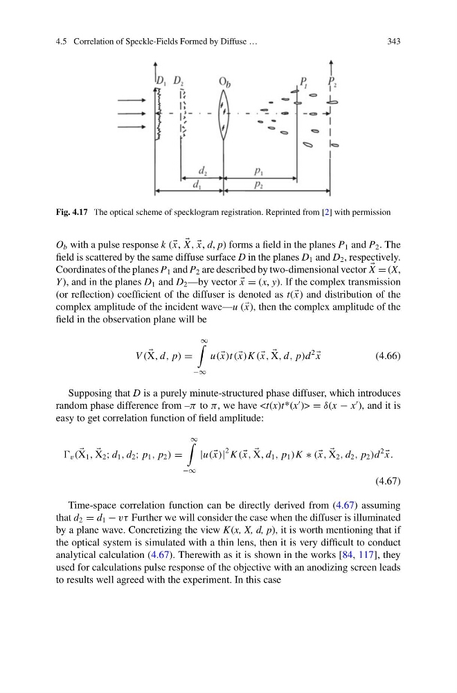
Fig. 4.17 The optical scheme of specklogram registration. Reprinted from [2] with permission
O b with a pulse response k ( x,
X ,
x, d, p) forms a field in the planes P 1 and P 2 . The
field is scattered by the same diffuse surface D in the planes D 1 and D 2 , respectively.
Coordinates of the planes P 1 and P 2 are described by two-dimensional vector
X = (X,
Y ), and in the planes D 1 and D 2 —by vector
x = (x, y). If the complex transmission
(or reflection) coefficient of the diffuser is denoted as t( x) and distribution of the
complex amplitude of the incident wave—u ( x), then the complex amplitude of the
field in the observation plane will be
V (
X, d, p) =
∞
−∞
u( x)t ( x)K ( x,
X, d, p)d
2
x
(4.66)
Supposing that D is a purely minute-structured phase diffuser, which introduces
random phase difference from –π to π, we have
), and it is
easy to get correlation function of field amplitude:
v (
X 1 ,
X 2 ; d 1 , d 2 ; p 1 , p 2 ) =
∞
−∞
|u( x)|
2 K ( x,
X, d 1 , p 1 )K ∗ ( x,
X 2 , d 2 , p 2 )d
2
x.
(4.67)
Time-space correlation function can be directly derived from (4.67) assuming
that d 2 = d 1 − vτ Further we will consider the case when the diffuser is illuminated
by a plane wave. Concretizing the view K(x, X, d, p), it is worth mentioning that if
the optical system is simulated with a thin lens, then it is very difficult to conduct
analytical calculation (4.67). Therewith as it is shown in the works [84, 117], they
used for calculations pulse response of the objective with an anodizing screen leads
to results well agreed with the experiment. In this case
343
Fig. 4.17 The optical scheme of specklogram registration. Reprinted from [2] with permission
O b with a pulse response k ( x,
X ,
x, d, p) forms a field in the planes P 1 and P 2 . The
field is scattered by the same diffuse surface D in the planes D 1 and D 2 , respectively.
Coordinates of the planes P 1 and P 2 are described by two-dimensional vector
X = (X,
Y ), and in the planes D 1 and D 2 —by vector
x = (x, y). If the complex transmission
(or reflection) coefficient of the diffuser is denoted as t( x) and distribution of the
complex amplitude of the incident wave—u ( x), then the complex amplitude of the
field in the observation plane will be
V (
X, d, p) =
∞
−∞
u( x)t ( x)K ( x,
X, d, p)d
2
x
(4.66)
Supposing that D is a purely minute-structured phase diffuser, which introduces
random phase difference from –π to π, we have
), and it is
easy to get correlation function of field amplitude:
v (
X 1 ,
X 2 ; d 1 , d 2 ; p 1 , p 2 ) =
∞
−∞
|u( x)|
2 K ( x,
X, d 1 , p 1 )K ∗ ( x,
X 2 , d 2 , p 2 )d
2
x.
(4.67)
Time-space correlation function can be directly derived from (4.67) assuming
that d 2 = d 1 − vτ Further we will consider the case when the diffuser is illuminated
by a plane wave. Concretizing the view K(x, X, d, p), it is worth mentioning that if
the optical system is simulated with a thin lens, then it is very difficult to conduct
analytical calculation (4.67). Therewith as it is shown in the works [84, 117], they
used for calculations pulse response of the objective with an anodizing screen leads
to results well agreed with the experiment. In this case