

324
4 Speckle-Optical Methods and Devices for Studying …
where
a =
π W
2
0
λ
,
(4.28)
a is the parameter, which determines the area of waist of the Gaussian beam; W 0
is the width of the beam in the area of waist.
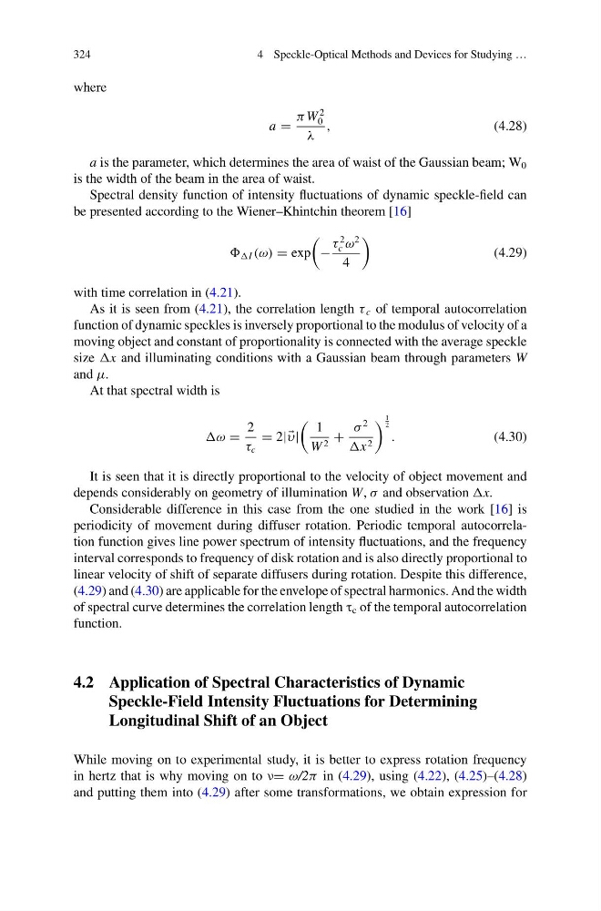
Spectral density function of intensity fluctuations of dynamic speckle-field can
be presented according to the Wiener–Khintchin theorem [16]
I (ω) = exp
−
τ
2
c ω
2
4
(4.29)
with time correlation in (4.21).
As it is seen from (4.21), the correlation length τ c of temporal autocorrelation
function of dynamic speckles is inversely proportional to the modulus of velocity of a
moving object and constant of proportionality is connected with the average speckle
size x and illuminating conditions with a Gaussian beam through parameters W
and μ.
At that spectral width is
ω =
2
τ c
= 2|
υ|
1
W 2 +
σ
2
x 2
1
2
.
(4.30)
It is seen that it is directly proportional to the velocity of object movement and
depends considerably on geometry of illumination W, σ and observation x.
Considerable difference in this case from the one studied in the work [16] is
periodicity of movement during diffuser rotation. Periodic temporal autocorrelation function gives line power spectrum of intensity fluctuations, and the frequency
interval corresponds to frequency of disk rotation and is also directly proportional to
linear velocity of shift of separate diffusers during rotation. Despite this difference,
(4.29) and (4.30) are applicable for the envelope of spectral harmonics. And the width
of spectral curve determines the correlation length τ c of the temporal autocorrelation
function.
4.2 Application of Spectral Characteristics of Dynamic
Speckle-Field Intensity Fluctuations for Determining
Longitudinal Shift of an Object
While moving on to experimental study, it is better to express rotation frequency
in hertz that is why moving on to ν= ω/2π in (4.29), using (4.22), (4.25)–(4.28)
and putting them into (4.29) after some transformations, we obtain expression for
4 Speckle-Optical Methods and Devices for Studying …
where
a =
π W
2
0
λ
,
(4.28)
a is the parameter, which determines the area of waist of the Gaussian beam; W 0
is the width of the beam in the area of waist.
Spectral density function of intensity fluctuations of dynamic speckle-field can
be presented according to the Wiener–Khintchin theorem [16]
I (ω) = exp
−
τ
2
c ω
2
4
(4.29)
with time correlation in (4.21).
As it is seen from (4.21), the correlation length τ c of temporal autocorrelation
function of dynamic speckles is inversely proportional to the modulus of velocity of a
moving object and constant of proportionality is connected with the average speckle
size x and illuminating conditions with a Gaussian beam through parameters W
and μ.
At that spectral width is
ω =
2
τ c
= 2|
υ|
1
W 2 +
σ
2
x 2
1
2
.
(4.30)
It is seen that it is directly proportional to the velocity of object movement and
depends considerably on geometry of illumination W, σ and observation x.
Considerable difference in this case from the one studied in the work [16] is
periodicity of movement during diffuser rotation. Periodic temporal autocorrelation function gives line power spectrum of intensity fluctuations, and the frequency
interval corresponds to frequency of disk rotation and is also directly proportional to
linear velocity of shift of separate diffusers during rotation. Despite this difference,
(4.29) and (4.30) are applicable for the envelope of spectral harmonics. And the width
of spectral curve determines the correlation length τ c of the temporal autocorrelation
function.
4.2 Application of Spectral Characteristics of Dynamic
Speckle-Field Intensity Fluctuations for Determining
Longitudinal Shift of an Object
While moving on to experimental study, it is better to express rotation frequency
in hertz that is why moving on to ν= ω/2π in (4.29), using (4.22), (4.25)–(4.28)
and putting them into (4.29) after some transformations, we obtain expression for