

24
2 Model of Quasi-Steady Weld Pool Dynamics and Numerical Simulation
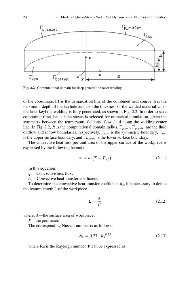
Fig. 2.2 Computational domain for deep penetration laser welding
of the coordinate. h1 is the demarcation line of the combined heat source. h is the
maximum depth of the keyhole and also the thickness of the welded material when
the laser keyhole welding is fully penetrated, as shown in Fig. 2.2. In order to save
computing time, half of the sheets is selected for numerical simulation, given the
symmetry between the temperature field and flow field along the welding center
line. In Fig. 2.2, R is the computational domain radius, p_out , , p_inlet are the fluid
outflow and inflow boundaries, respectively, sym is the symmetric boundary, top
is the upper surface boundary, and bottom is the lower surface boundary.
The convective heat loss per unit area of the upper surface of the workpiece is
expressed by the following formula:
q c = h c
T − T re f
(2.11)
In this equation:
q c —Convective heat flux;
h c —Convective heat transfer coefficient.
To determine the convective heat transfer coefficient h c , it is necessary to define
the feature length L of the workpiece.
L =
A
P
(2.12)
where: A—the surface area of workpiece;
P—the perimeter.
The corresponding Nusselt number is as follows:
N u = 0.27 · R a
0.25
(2.13)
where Ra is the Rayleigh number. It can be expressed as:
2 Model of Quasi-Steady Weld Pool Dynamics and Numerical Simulation
Fig. 2.2 Computational domain for deep penetration laser welding
of the coordinate. h1 is the demarcation line of the combined heat source. h is the
maximum depth of the keyhole and also the thickness of the welded material when
the laser keyhole welding is fully penetrated, as shown in Fig. 2.2. In order to save
computing time, half of the sheets is selected for numerical simulation, given the
symmetry between the temperature field and flow field along the welding center
line. In Fig. 2.2, R is the computational domain radius, p_out , , p_inlet are the fluid
outflow and inflow boundaries, respectively, sym is the symmetric boundary, top
is the upper surface boundary, and bottom is the lower surface boundary.
The convective heat loss per unit area of the upper surface of the workpiece is
expressed by the following formula:
q c = h c
T − T re f
(2.11)
In this equation:
q c —Convective heat flux;
h c —Convective heat transfer coefficient.
To determine the convective heat transfer coefficient h c , it is necessary to define
the feature length L of the workpiece.
L =
A
P
(2.12)
where: A—the surface area of workpiece;
P—the perimeter.
The corresponding Nusselt number is as follows:
N u = 0.27 · R a
0.25
(2.13)
where Ra is the Rayleigh number. It can be expressed as: