

100
3 Coupling Model and Numerical Computation Method of Keyhole and Weld Pool
where:
− →
U
∗
Intermediate velocity field;
C(·),
D(·),
K (·) and
F
n
Mathematical operators for convection terms, viscous
terms, Darcy terms, and buoyancy terms in discrete
momentum conservation equation.
In order to improve the accuracy of the numerical calculation, the fifth-order
WENO scheme is used to discretize the operator in this study
C
− →
U
n
, and in order
to facilitate the loading of the viscous stress boundary conditions caused by thermal
capillary force (see Eq. (3.56)), the second-order central difference format is used
to discretize the viscosity term
D
− →
U
n
. At the same time, in order to speed up
the calculation, both Darcy and buoyancy terms are discretized using the explicit
scheme. In particular, the loading of viscous stress boundary conditions on a staggered difference grid is very complicated and will be discussed in detail in the next
section. Besides, there will be certain requirements on the time step if both Darcy
and buoyancy terms are explicitly processed, which will be discussed in more details
in the subsequent chapters.
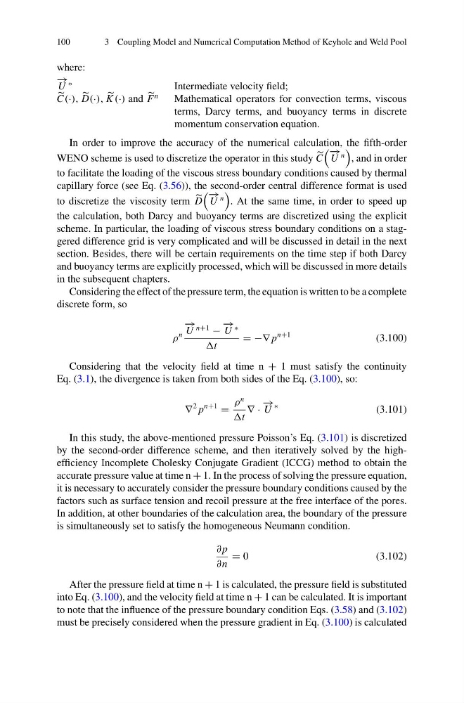
Considering the effect of the pressure term, the equation is written to be a complete
discrete form, so
ρ
n
− →
U
n+1
−
− →
U
∗
t
= −∇ p
n+1
(3.100)
Considering that the velocity field at time n + 1 must satisfy the continuity
Eq. (3.1), the divergence is taken from both sides of the Eq. (3.100), so:
∇
2 p
n+1
=
ρ
n
t
∇ ·
− →
U
∗
(3.101)
In this study, the above-mentioned pressure Poisson’s Eq. (3.101) is discretized
by the second-order difference scheme, and then iteratively solved by the highefficiency Incomplete Cholesky Conjugate Gradient (ICCG) method to obtain the
accurate pressure value at time n + 1. In the process of solving the pressure equation,
it is necessary to accurately consider the pressure boundary conditions caused by the
factors such as surface tension and recoil pressure at the free interface of the pores.
In addition, at other boundaries of the calculation area, the boundary of the pressure
is simultaneously set to satisfy the homogeneous Neumann condition.
∂ p
∂n
= 0
(3.102)
After the pressure field at time n + 1 is calculated, the pressure field is substituted
into Eq. (3.100), and the velocity field at time n + 1 can be calculated. It is important
to note that the influence of the pressure boundary condition Eqs. (3.58) and (3.102)
must be precisely considered when the pressure gradient in Eq. (3.100) is calculated
3 Coupling Model and Numerical Computation Method of Keyhole and Weld Pool
where:
− →
U
∗
Intermediate velocity field;
C(·),
D(·),
K (·) and
F
n
Mathematical operators for convection terms, viscous
terms, Darcy terms, and buoyancy terms in discrete
momentum conservation equation.
In order to improve the accuracy of the numerical calculation, the fifth-order
WENO scheme is used to discretize the operator in this study
C
− →
U
n
, and in order
to facilitate the loading of the viscous stress boundary conditions caused by thermal
capillary force (see Eq. (3.56)), the second-order central difference format is used
to discretize the viscosity term
D
− →
U
n
. At the same time, in order to speed up
the calculation, both Darcy and buoyancy terms are discretized using the explicit
scheme. In particular, the loading of viscous stress boundary conditions on a staggered difference grid is very complicated and will be discussed in detail in the next
section. Besides, there will be certain requirements on the time step if both Darcy
and buoyancy terms are explicitly processed, which will be discussed in more details
in the subsequent chapters.
Considering the effect of the pressure term, the equation is written to be a complete
discrete form, so
ρ
n
− →
U
n+1
−
− →
U
∗
t
= −∇ p
n+1
(3.100)
Considering that the velocity field at time n + 1 must satisfy the continuity
Eq. (3.1), the divergence is taken from both sides of the Eq. (3.100), so:
∇
2 p
n+1
=
ρ
n
t
∇ ·
− →
U
∗
(3.101)
In this study, the above-mentioned pressure Poisson’s Eq. (3.101) is discretized
by the second-order difference scheme, and then iteratively solved by the highefficiency Incomplete Cholesky Conjugate Gradient (ICCG) method to obtain the
accurate pressure value at time n + 1. In the process of solving the pressure equation,
it is necessary to accurately consider the pressure boundary conditions caused by the
factors such as surface tension and recoil pressure at the free interface of the pores.
In addition, at other boundaries of the calculation area, the boundary of the pressure
is simultaneously set to satisfy the homogeneous Neumann condition.
∂ p
∂n
= 0
(3.102)
After the pressure field at time n + 1 is calculated, the pressure field is substituted
into Eq. (3.100), and the velocity field at time n + 1 can be calculated. It is important
to note that the influence of the pressure boundary condition Eqs. (3.58) and (3.102)
must be precisely considered when the pressure gradient in Eq. (3.100) is calculated