

3.5 Numerical Method
99
3.5.3.1 Projection Method for Solving the Flow Field of the Motion
Weld Pool
As an efficient step-by-step method for solving the incompressible Navier–Stokes
equation, an outstanding advantage of the Projection method is that when the Navier–
Stokes equation is being solved, the velocity and the pressure are decoupled during
the solution. The Projection method is based on the well-known Helmholtz-Hodege
decomposition principle: that is to say, any vector field can always be decomposed
into a Solenoidal part and an Irrotational part. In general, the incompressible Navier–
Stokes equation being solved by the Projection method can be divided into three
steps: the first step is to calculate an intermediate velocity field that does not meet
the incompressible condition; the second step is to use the intermediate velocity field
to calculate the pressure field of the next moment; at last, the intermediate velocity
field is projected into a velocity space with zero divergence by using the pressure, to
obtain an accurate velocity field. The procedure for solving the coupled Eqs. (3.1) and
(3.2) using the Projection method based on the staggered difference grid technique
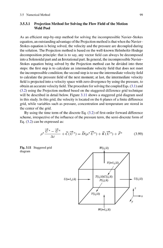
will be described in detail below. Figure 3.11 shows a staggered grid diagram used
in this study. In this grid, the velocity is located on the 6 planes of a finite difference
grid, while variables such as pressure, concentration and temperature are stored in
the center of the grid.
By using the time term of the discrete Eq. (3.2) of first-order forward difference
scheme, irrespective of the influence of the pressure term, the semi-discrete form of
Eq. (3.2) can be expressed as:
ρ
n
− →
U
∗
−
− →
U
n
t
+
C(
− →
U
n
) =
D(μ
n − →
U
n
) +
K (
− →
U
n
) +
F
n
(3.99)
Fig. 3.11 Staggered grid
diagram
99
3.5.3.1 Projection Method for Solving the Flow Field of the Motion
Weld Pool
As an efficient step-by-step method for solving the incompressible Navier–Stokes
equation, an outstanding advantage of the Projection method is that when the Navier–
Stokes equation is being solved, the velocity and the pressure are decoupled during
the solution. The Projection method is based on the well-known Helmholtz-Hodege
decomposition principle: that is to say, any vector field can always be decomposed
into a Solenoidal part and an Irrotational part. In general, the incompressible Navier–
Stokes equation being solved by the Projection method can be divided into three
steps: the first step is to calculate an intermediate velocity field that does not meet
the incompressible condition; the second step is to use the intermediate velocity field
to calculate the pressure field of the next moment; at last, the intermediate velocity
field is projected into a velocity space with zero divergence by using the pressure, to
obtain an accurate velocity field. The procedure for solving the coupled Eqs. (3.1) and
(3.2) using the Projection method based on the staggered difference grid technique
will be described in detail below. Figure 3.11 shows a staggered grid diagram used
in this study. In this grid, the velocity is located on the 6 planes of a finite difference
grid, while variables such as pressure, concentration and temperature are stored in
the center of the grid.
By using the time term of the discrete Eq. (3.2) of first-order forward difference
scheme, irrespective of the influence of the pressure term, the semi-discrete form of
Eq. (3.2) can be expressed as:
ρ
n
− →
U
∗
−
− →
U
n
t
+
C(
− →
U
n
) =
D(μ
n − →
U
n
) +
K (
− →
U
n
) +
F
n
(3.99)
Fig. 3.11 Staggered grid
diagram