

94
3 Coupling Model and Numerical Computation Method of Keyhole and Weld Pool
After updating or re-initializing the position of each step of Level Set function,
the value of the Level Set function needs to be corrected with the information of
particles. The basis for the correction is that if the particle that started on the positive
side of the interface goes to the negative side of the interface, then the Level Set
function shall be corrected; conversely, if the particle with a negative distance value
goes to the side with a positive distance value, a correction shall be conducted.
The most difficult part of adopting the Particle Level Set method is the increase,
deletion and re-seeding of particles. In the process of numerical calculation, due
to the influence of numerical error at the interface, the previously seeded particles
need to be deleted and re-seeded at a specific time. Obviously, there is no prescribed
rule about when to delete a particle and re-seed one. This is only related to specific
problems. In this study, it is stipulated that all particles shall be deleted and re-seeded
every certain computational time step. Besides, when the area of the tracked interface
changes greatly, it may be needed to add some particles to correct the dissipation of
the Level Set values. When the Level Set is used to track the interface, the surface
area of the interface can be accurately determined according to the following formula
S =
δ(ϕ)|∇ϕ|dV
(3.96)
where δ(ϕ)—Dirac function, which only has a value on the interface, and the value
is 1; and the value is 0 at any other position.
In this study, it is stipulated that when the area of the current interface is compared
with the area in the last particle seeding, once the ratio is larger than a certain critical
value, a certain number of particles will be appropriately added on both sides of the
interface on the original basis.
3.5.2.3 Numerical Examples
To verify the rationality of the Level Set and Particle Level Set interface tracking
technologies developed by the institute, two classical numerical examples, namely,
the shear flow field and notched Zalesak disc, are used to test the interface tracking
technologies developed by the institute respectively.
The example of shear flow field is mainly used to test the interface tracking
method, to check the mass conservation of the interface when the interface has shear
deformation in the flow field. The disc radius may as well be set to be 15, and the
center of the circle is at (5,75). The flow function of the flow field is
ψ =
1
π
sin
2
(π x) sin
2
(π y)
(3.97)
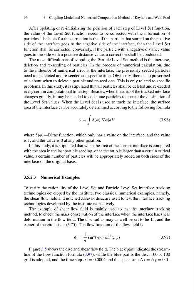
Figure 3.5 shows the disc and shear flow field. The black part indicates the streamline of the flow function formula (3.97), while the blue part is the disc. 100 × 100
grid is adopted, and the time step t = 0.0004 and the space step x = y = 0.01
3 Coupling Model and Numerical Computation Method of Keyhole and Weld Pool
After updating or re-initializing the position of each step of Level Set function,
the value of the Level Set function needs to be corrected with the information of
particles. The basis for the correction is that if the particle that started on the positive
side of the interface goes to the negative side of the interface, then the Level Set
function shall be corrected; conversely, if the particle with a negative distance value
goes to the side with a positive distance value, a correction shall be conducted.
The most difficult part of adopting the Particle Level Set method is the increase,
deletion and re-seeding of particles. In the process of numerical calculation, due
to the influence of numerical error at the interface, the previously seeded particles
need to be deleted and re-seeded at a specific time. Obviously, there is no prescribed
rule about when to delete a particle and re-seed one. This is only related to specific
problems. In this study, it is stipulated that all particles shall be deleted and re-seeded
every certain computational time step. Besides, when the area of the tracked interface
changes greatly, it may be needed to add some particles to correct the dissipation of
the Level Set values. When the Level Set is used to track the interface, the surface
area of the interface can be accurately determined according to the following formula
S =
δ(ϕ)|∇ϕ|dV
(3.96)
where δ(ϕ)—Dirac function, which only has a value on the interface, and the value
is 1; and the value is 0 at any other position.
In this study, it is stipulated that when the area of the current interface is compared
with the area in the last particle seeding, once the ratio is larger than a certain critical
value, a certain number of particles will be appropriately added on both sides of the
interface on the original basis.
3.5.2.3 Numerical Examples
To verify the rationality of the Level Set and Particle Level Set interface tracking
technologies developed by the institute, two classical numerical examples, namely,
the shear flow field and notched Zalesak disc, are used to test the interface tracking
technologies developed by the institute respectively.
The example of shear flow field is mainly used to test the interface tracking
method, to check the mass conservation of the interface when the interface has shear
deformation in the flow field. The disc radius may as well be set to be 15, and the
center of the circle is at (5,75). The flow function of the flow field is
ψ =
1
π
sin
2
(π x) sin
2
(π y)
(3.97)
Figure 3.5 shows the disc and shear flow field. The black part indicates the streamline of the flow function formula (3.97), while the blue part is the disc. 100 × 100
grid is adopted, and the time step t = 0.0004 and the space step x = y = 0.01