

90
4 Application of the Set-Theoretic Algorithm to CFRP’s
Table 4.1 Summary of electrical properties of some composites [5]
Graphite-Epoxy
Boron-Epoxy
Kevlar
Permeability (μ R )
1
1
1
Permittivity ( R )
Indeterminate
5.6
3.6
DC conductivity (S/m)
Longitudinal (σ L )
2 × 10 4
30
6 × 10 −9
Transverse (σ T )
100
2 × 10 −8
6 × 10 −9
Anisotropy ratio (σ L /σ T )
200
1.5 × 10 9
1
-4x10
6
-3x10
6
-2x10
6
-1x10
6
0
1x10
6
2x10
6
3x10
6
4x10
6
5x10
6
-200 -150 -100 -50
0
50 100 150 200 250
Jx
Ex
Anomalous Conductivity for (k,l,m) = (3,3,1)
Real
Imag
Jx = 19.900E+03*Ex
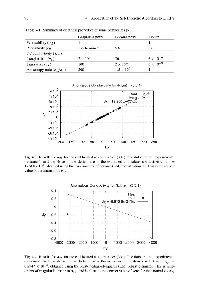
Fig. 4.3 Results for σ xx for the cell located at coordinates (331). The dots are the ‘experimental
outcomes’, and the slope of the dotted line is the estimated anomalous conductivity, σ xx =
19.900×10 3 , obtained using the least-median-of-squares (LM) robust estimator. This is the correct
value of the anomalous σ xx
-0.8
-0.6
-0.4
-0.2
0
0.2
0.4
-4000 -3000 -2000 -1000
0
1000 2000 3000 4000
Jy
Ey
Anomalous Conductivity for (k,l,m) = (3,3,1)
Real
Imag
Jy = -0.9731E-04*Ey
Fig. 4.4 Results for σ yy for the cell located at coordinates (331). The dots are the ‘experimental
outcomes’, and the slope of the dotted line is the estimated anomalous conductivity, σ yy =
0.2947 × 10 −4 , obtained using the least-median-of-squares (LM) robust estimator. This is nineorders of magnitude less than σ xx , and is close to the correct value of zero for the anomalous σ yy
4 Application of the Set-Theoretic Algorithm to CFRP’s
Table 4.1 Summary of electrical properties of some composites [5]
Graphite-Epoxy
Boron-Epoxy
Kevlar
Permeability (μ R )
1
1
1
Permittivity ( R )
Indeterminate
5.6
3.6
DC conductivity (S/m)
Longitudinal (σ L )
2 × 10 4
30
6 × 10 −9
Transverse (σ T )
100
2 × 10 −8
6 × 10 −9
Anisotropy ratio (σ L /σ T )
200
1.5 × 10 9
1
-4x10
6
-3x10
6
-2x10
6
-1x10
6
0
1x10
6
2x10
6
3x10
6
4x10
6
5x10
6
-200 -150 -100 -50
0
50 100 150 200 250
Jx
Ex
Anomalous Conductivity for (k,l,m) = (3,3,1)
Real
Imag
Jx = 19.900E+03*Ex
Fig. 4.3 Results for σ xx for the cell located at coordinates (331). The dots are the ‘experimental
outcomes’, and the slope of the dotted line is the estimated anomalous conductivity, σ xx =
19.900×10 3 , obtained using the least-median-of-squares (LM) robust estimator. This is the correct
value of the anomalous σ xx
-0.8
-0.6
-0.4
-0.2
0
0.2
0.4
-4000 -3000 -2000 -1000
0
1000 2000 3000 4000
Jy
Ey
Anomalous Conductivity for (k,l,m) = (3,3,1)
Real
Imag
Jy = -0.9731E-04*Ey
Fig. 4.4 Results for σ yy for the cell located at coordinates (331). The dots are the ‘experimental
outcomes’, and the slope of the dotted line is the estimated anomalous conductivity, σ yy =
0.2947 × 10 −4 , obtained using the least-median-of-squares (LM) robust estimator. This is nineorders of magnitude less than σ xx , and is close to the correct value of zero for the anomalous σ yy